Predicting Next Day Rain In Australia
Table Of Contents:
- What Is The Business Use Case?
- Python Implementation.
(1) What Is The Business Use Case ?
- Predicting next day rain using a dataset containing 10 years of daily weather observations from different location across Australia.

(2) Python Implementation.
(1) Importing Required Library
import matplotlib.pyplot as plt
import seaborn as sns
import datetime
from sklearn import preprocessing
from sklearn.preprocessing import LabelEncoder
from sklearn.preprocessing import StandardScaler
from sklearn.model_selection import train_test_split
from keras.layers import Dense, BatchNormalization, Dropout, LSTM
from keras.model import Sequential
from keras.utils import to_categorical
from keras.optimizer import Adam
from tensorflow.keras import regularizers
from keras import callbacks
from sklearn.metrics import precision_score, recall_score, confusion_matrix, classification_report, accuracy_score, f1_score
np.random.seed(0)
(2) Data Loading
data = pd.read_csv('weatherAUS.csv')
data.head()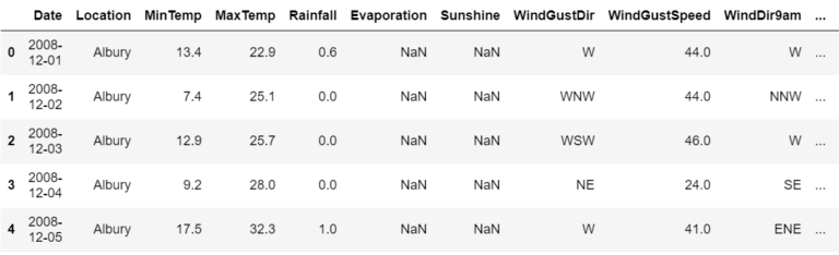
The dataset contains about 10 years of daily weather observations from different locations across Australia.
Observations were drawn from numerous weather stations.
In this project, I will use this data to predict whether or not it will rain the next day.
There are 23 attributes including the target variable “RainTomorrow”, indicating whether or not it will rain the next day or not.
(3) Data Information
data.info()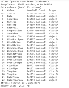
- There are missing values in the dataset
- Dataset includes numeric and categorical values.
(4) Data Visualization & Cleaning
- Steps involved in this section.
- Count plot of target column
- Correlation amongst numeric attributes
- Parse Dates into datetime
- Encoding days and months as continuous cyclic features.
First of all let us evaluate the target and find out if our data is imbalanced or not?
cols = ['blue','red']
sns.countplot(x=data['RainTomorrow'], palette=cols)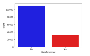
Correlation amongst numeric attributes
corrmat = data.corr()
cmap = sns.diverging_palette(260,-10,s=50, l=75, n=6, as_cmap=True)
plt.subplots(figsize=(18,18))
sns.heatmap(corrmat,cmap=cmap, annot=True, square=True)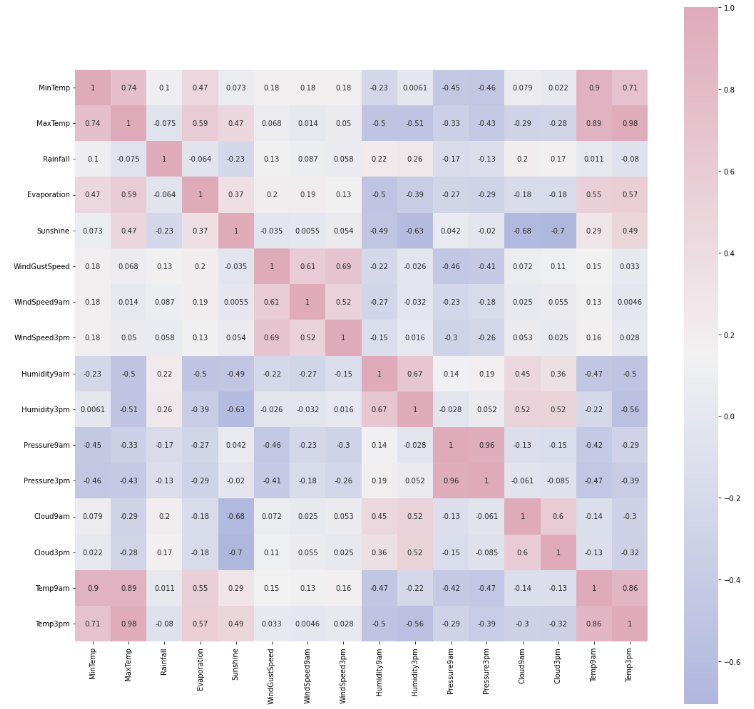
Parsing Dates Into DateTime Object.
- My goal is to build an artificial neural network(ANN). I will encode dates appropriately, i.e. I prefer the months and days in a cyclic continuous feature.
- A date and time are inherently cyclical.
- To let the ANN model know that a feature is cyclical I split it into periodic subsections.
- Namely, years, months and days. Now for each subsection, I create two new features, deriving a sine and cosine transformations of the subsection feature.
Exploring the length of date objects
lengths = data['Date'].str.len()
lengths.value_counts()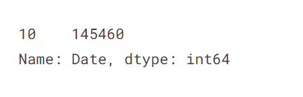
- There doesn’t seem to be any missing values in dates so parsing values into datetime
Converting The Date Object To The DateTime Format:
data['Date'] = pd.to_datetime(date['Date'])Creating A New Column For Year:
data['year'] = data.Date.dt.yearFunction to encode datetime into cyclic parameters.
def encode(data, col, max_val):
    data[col + '_sin'] = np.sin(2 * np.pi * data[col]/max_val)
    data[col + '_cos'] = np.cos(2 * np.pi * data[col]/max_val)
    return data
data['month'] = data.Date.dt.month
data = encode(data, 'month', 12)
data['day'] = data.Date.dt.day
data = encode(data, 'day', 31)
data.head()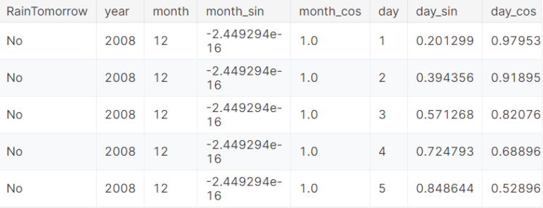
Plotting Distribution Of Days Over Years:
section = data[:360]
tm = section["day"].plot(color="#C2C4E2")
tm.set_title("Distribution Of Days Over Year")
tm.set_ylabel("Days In month")
tm.set_xlabel("Days In Year")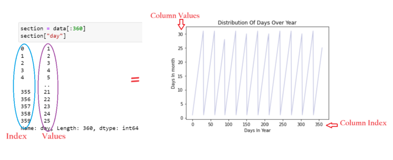
- As expected, the “year” attribute of data repeats.
- However, in this, the true cyclic nature is not presented in a continuous manner.
- Splitting months and days into Sine and cosine combinations provides the cyclical continuous feature.
- This can be used as input features to ANN.
cyclic_month = sns.scatterplot(x='month_sin', y='month_cos', data=data, color="#C2C4E2")
cyclic_month.set_title("Cyclic Encoding of Month")
cyclic_month.set_ylabel("Cosine Encoded Months")
cyclic_month.set_xlabel("Sine Encoded Months")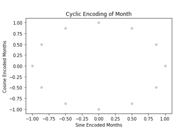
- To implement the true nature of the date column we need to split the date column into sine and cosine terms.
- We need to combine both the sine and cosine terms to implement the cyclic nature of date and month column.
cyclic_day = sns.scatterplot(x='day_sin',y='day_cos',data=data, color="#C2C4E2")
cyclic_day.set_title("Cyclic Encoding of Day")
cyclic_day.set_ylabel("Cosine Encoded Day")
cyclic_day.set_xlabel("Sine Encoded Day")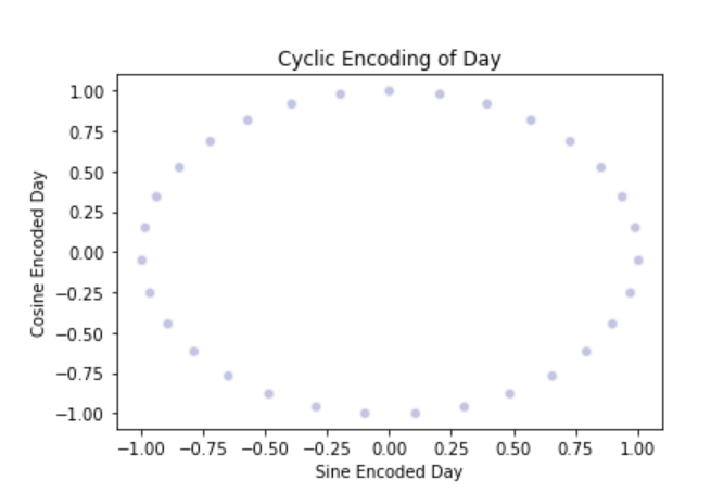
Next, I will deal with missing values in categorical and numeric attributes separately
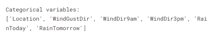
Categorical Variable:
- Filling missing value with the mode of the column.
- Get the list of categorical variables.
s = (data.dtypes == 'object')
object_cols = list(s[s].index)
print('Categorical Variables:')
print(object_cols)
Missing Values In Categorical Columns:
for i in object_cols:
    print(i, data[i].isnull().sum())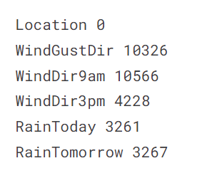
Filling missing values with mode of the column in value:
for i in object_cols:
    data[i].fillna(data[i].mode()[0], inplace=True)
Numerical Variables:
- Filling missing value with the median of the column.
- Get the list of numeric variables.
t = (data.dtypes == 'float64')
num_cols = list(t[t].index)

print('Numeric Variables:')
print(num_cols)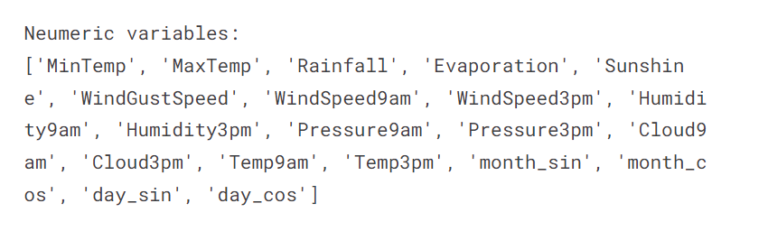
Missing Values In Numeric Columns:
for i in num_cols:
    print(i, data[i].isnull().sum)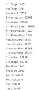
Filling missing values with median of the column in value:
for i in object_cols:
    data[i].fillna(data[i].median()[0], inplace=True)
data.info()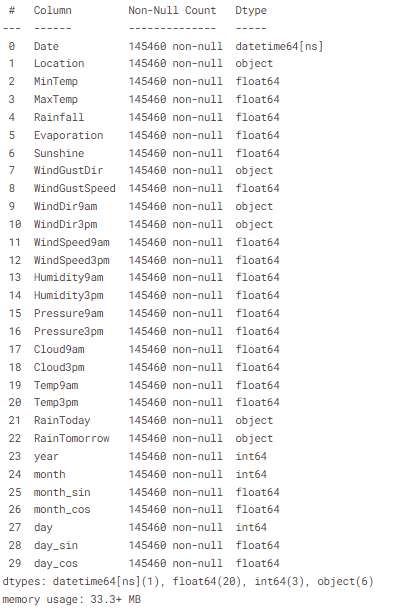
(5) Data Preprocessing
- Label encoding columns with categorical data.
- Perform the scaling of the features.
- Detecting outliers.
- Dropping the outliers based on data analysis.
Label Encoding The Categorical Variable:
label_encoder = LabelEncoder()

for i in object_cols:
    data[i] = label_encoder.fit_transform(data[i])

data[object_cols]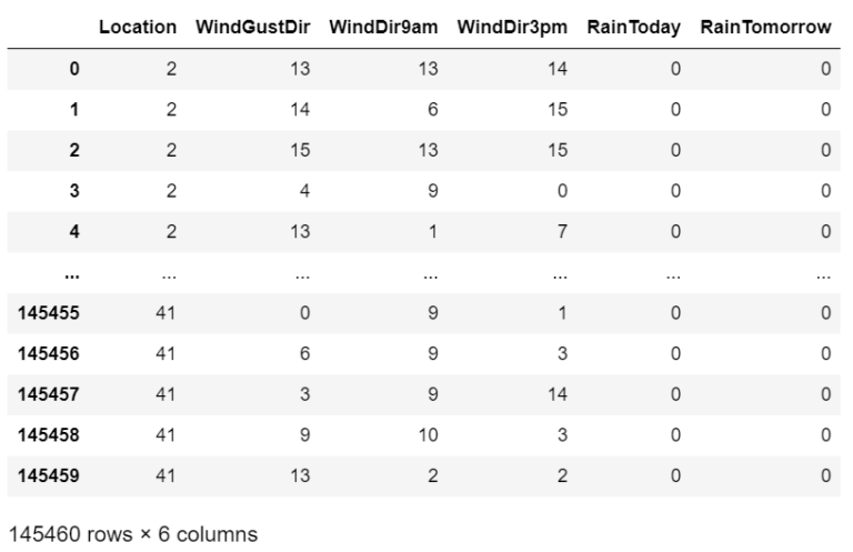
Standardizing The Numerical Variables:
# Dropping Target & Extra Columns
features = data.drop(['RainTomorrow', 'Date', 'day', 'month'], axis=1)
# Creating The Target Column
target = data['RainTomorrow']
col_names = list(features.columns)
s_scalar = preprocessing.StandardScalar()
features = s_scalar.fit_transform(features)
features = pd.DataFrame(features, columns=col_names)
features.head()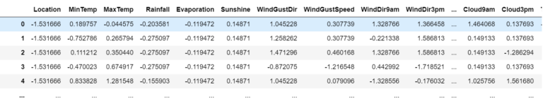
Outlier Detection:
colours = ["#D0DBEE", "#C2C4E2", "#EED4E5", "#D1E6DC", "#BDE2E2"]
plt.figure(figsize=(20,10))

sns.boxenplot(data = features, palette = colours)
plt.xticks(rotations=90)
plt.show()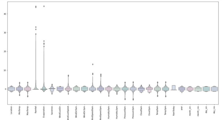
# Adding The Target Variable
features["RainTomorrow"] = target

# Dropping The Outlier values
features = features[(features["MinTemp"]<2.3)&(features["MinTemp"]>-2.3)]
features = features[(features["MaxTemp"]<2.3)&(features["MaxTemp"]>-2)]
features = features[(features["Rainfall"]<4.5)]
features = features[(features["Evaporation"]<2.8)]
features = features[(features["Sunshine"]<2.1)]
features = features[(features["WindGustSpeed"]<4)&(features["WindGustSpeed"]>-4)]
features = features[(features["WindSpeed9am"]<4)]
features = features[(features["WindSpeed3pm"]<2.5)]
features = features[(features["Humidity9am"]>-3)]
features = features[(features["Humidity3pm"]>-2.2)]
features = features[(features["Pressure9am"]< 2)&(features["Pressure9am"]>-2.7)]
features = features[(features["Pressure3pm"]< 2)&(features["Pressure3pm"]>-2.7)]
features = features[(features["Cloud9am"]<1.8)]
features = features[(features["Cloud3pm"]<2)]
features = features[(features["Temp9am"]<2.3)&(features["Temp9am"]>-2)]
features = features[(features["Temp3pm"]<2.3)&(features["Temp3pm"]>-2)]
features.shape
Looking at the scaled features without outliers
plt.figure(figsize=(20,10))
sns.boxenplot(data=features, palette=colours)
plt.xticks(rotation=90)
plt.show()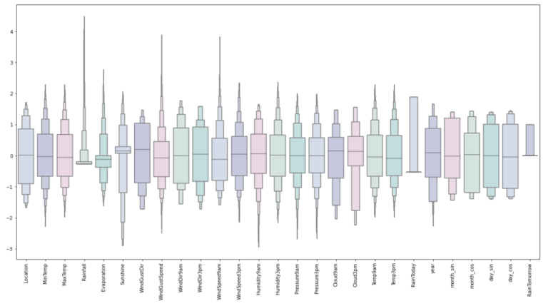
- Looks Good.
- Up next is building an Artificial Neural Network.
(6) Model Building
- Assigning ‘X’ and ‘y’ the status of attributes and tags
- Splitting test and training sets
- Initialising the neural network
- Defining by adding layers
- Compiling the neural network
- Train the neural network
Assigning X and y the status of attributes and tags:
X = features.drop(['RainTomorrow'], axis=1)
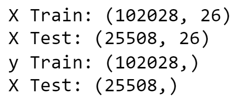
y = features['RainTomorrow']Splitting Test And Training Sets:
X_train, X_test, y_train, y_test = train_test_split(X, y, test_size = 0.2, random_state = 2)

print('X Train:', X_train.shape)
print('X Test:',  X_test.shape)
print('y Train:', y_train.shape)
print('X Test:', y_test.shape)
Defining Early Stopping Method:
early_stopping = callbacks.EarlyStopping(
    min_delta=0.001, # minimium amount of change to count as an improvement
    patience=20, # how many epochs to wait before stopping
    restore_best_weights=True,
)
Initializing the Neural Networks:
model = Sequential()Defining The Neural Network Layers:
model.add(Dense(units = 32, kernel_initializer = 'uniform', activation = 'relu', input_dim = 26))

model.add(Dense(units = 32, kernel_initializer = 'uniform', activation = 'relu'))

model.add(Dense(units=16, kernel_initializer = 'uniform', activation = 'relu'))

model.add(Dropout(0.25))

model.add(Dense(units = 8, kernel_initializer = 'uniform', activation = 'relu'))

model.add(Dropout(0.5))

model.add(Dense(units=1, kernel_initializer = 'uniform', activation = 'relu'))
Compiling The ANN:
opt = Adam(learning_rate = 0.00009)
model.compile(optimizer = opt, loss = 'binary_crossentropy', metrics = ['accuracy'])
Training ANN Model:
history = model.fit(X_train, y_train, batch_size = 32, epochs = 150, callbacks = [early_stopping], validation_split = 0.2)Plotting Training & Validation Loss Over Epochs:
history_df = pd.DataFrame(history.history)

plt.plot(history_df.loc[:, ['loss']], "#BDE2E2", label='Training loss')
plt.plot(history_df.loc[:, ['val_loss']],"#C2C4E2", label='Validation loss')
plt.title('Training and Validation loss')
plt.xlabel('Epochs')
plt.ylabel('Loss')
plt.legend(loc="best")

plt.show()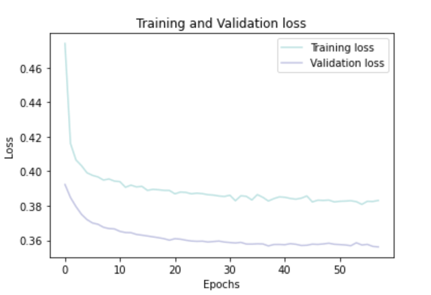
Plotting Training And Validation Accuracy Over Epochs:
history_df = pd.DataFrame(history.history)

plt.plot(history_df.loc[:, ['accuracy']], "#BDE2E2", label='Training accuracy')
plt.plot(history_df.loc[:, ['val_accuracy']], "#C2C4E2", label='Validation accuracy')

plt.title('Training and Validation accuracy')
plt.xlabel('Epochs')
plt.ylabel('Accuracy')
plt.legend()
plt.show()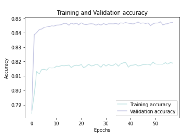
(7) Conclusion:
- Testing on the test set.
- Evaluating the confusion matrix.
- Evaluating the classification report.
Predicting The Test Set Result:
y_pred = model.predict(X_test)
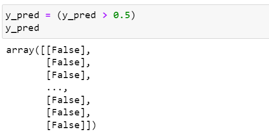
y_pred = (y_pred > 0.5)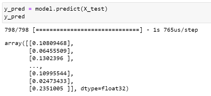
Predicting Confusion Matrix:
cmap1 = sns.diverging_palette(260,-10,s=50, l=75, n=5, as_cmap=True)
plt.subplots(figsize=(12,8))
cf_matrix = confusion_matrix(y_test, y_pred)
sns.heatmap(cf_matrix/np.sum(cf_matrix), cmap = cmap1, annot = True, annot_kws = {'size':15})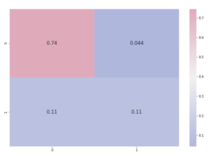
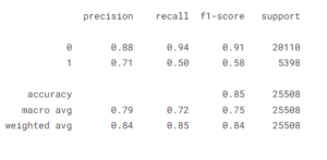
Predicting Classification Report
print(classification_report(y_test, y_pred))