
Image Classification With ANN!
Table Of Contents:
- What Is The Business Use Case?
- Importing Required Libraries.
- Loading Data.
- Shape Of Data.
- Data Types Of Dataset.
- Creating Validation Data And Scaling Data To Range (0-1).
- Looking At The First Two Images.
- Validation and Test Set Size.
- Let’s Look At A Sample Of The Images In The Dataset.
- Model Building.
- Compiling The Image Classification Model.
- Training & Evaluating Image Classification Model.
- Model Evaluation.
- Model Visualization.
- Visualizing Training And Validation Loss.
- Visualizing Training And Validation Accuracy.
- Making Prediction.
- Confusion Matrix.
- Looking At Some Random Prediction.
- Use The Model To Make Prediction.
- Here, the classification model classifies all five images correctly.
(1) What Is The Business Use case ?
- Image classification of the products.

(2) Importing Required Libraries
import pandas as pd
import numpy as np
import seaborn as sns
import matplotlib.pyplot as plt

import tensorflow as tf
from tensorflow import keras
from keras.models import Sequential
from keras.layers import Dense
(3) Loading Data
fashion_mnist = tf.keras.datasets.fashion_mnist
(X_train, y_train), (X_test, y_test) = fashion_mnist.load_data()
(4) Shape Of Data
X_train.shape, X_test.shape, y_train.shape, y_test.shape
(5) Data Types Of Dataset
X_train.dtype, X_test.dtype, y_train.dtype, y_test.dtype
(6) Creating Validation Data And Scaling Data To Range (0-1)
X_valid, X_train = X_train[:4000], X_train[4000:] / 255
y_valid, y_train = y_train[:4000], y_train[4000:]
X_test = X_test / 255
(7) Looking At The First Two Images
plt.figure(figsize = (15, 4))
plotnumber = 1

for i in range(2):
    if plotnumber <= 2:
        ax = plt.subplot(1, 2, plotnumber)
        plt.imshow(X_train[i], cmap = 'binary')
        plt.axis('off')

    plotnumber += 1

plt.tight_layout()
plt.show()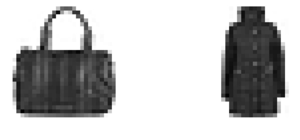
y_train
class_names = ["T-shirt/top", "Trouser", "Pullover", "Dress", "Coat",
               "Sandal", "Shirt", "Sneaker", "Bag", "Ankle boot"]
class_names[y_train[0]], class_names[y_train[1]] (8) Validation & Test Set Size
X_valid.shape
X_test.shape
(9) Let’s Take A Look At A Sample Of The Images In The Dataset:
plt.figure(figsize = (15, 6))
plotnumber = 1

for i in range(51):
    if plotnumber <= 50:
        ax = plt.subplot(5, 10, plotnumber)
        plt.imshow(X_train[i], cmap = 'binary')
        plt.axis('off')
        plt.title(class_names[y_train[i]], fontdict = {'fontsize'  : 12, 'color' : 'black'})

    plotnumber += 1

plt.tight_layout()
plt.show()
(9) Model Building
model = keras.models.Sequential([
    keras.layers.Flatten(input_shape = [28, 28]),
    keras.layers.Dense(100, activation = 'relu'),
    keras.layers.Dense(70, activation = 'relu'),
    keras.layers.Dense(50, activation = 'relu'),
    keras.layers.Dense(20, activation = 'relu'),
    keras.layers.Dense(10, activation = 'softmax')
])
model.summary()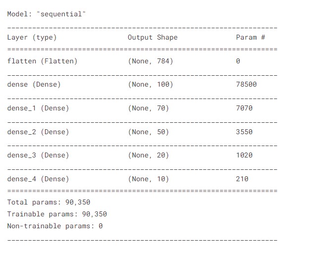
(10) Compiling The Image Classification Model
model.compile(loss = tf.keras.losses.SparseCategoricalCrossentropy(),
              optimizer = tf.keras.optimizers.Adam(), metrics = ['accuracy'])
(11) Training & Evaluating Image Classification Model
model_history = model.fit(X_train, y_train, validation_data = (X_valid, y_valid), epochs = 50)
(12) Model Evaluation:
model.evaluate(X_test, y_test)
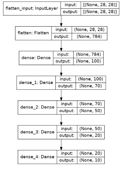
(13) Model Visualization
from tensorflow.keras.utils import plot_model

plot_model(model, show_shapes = True)
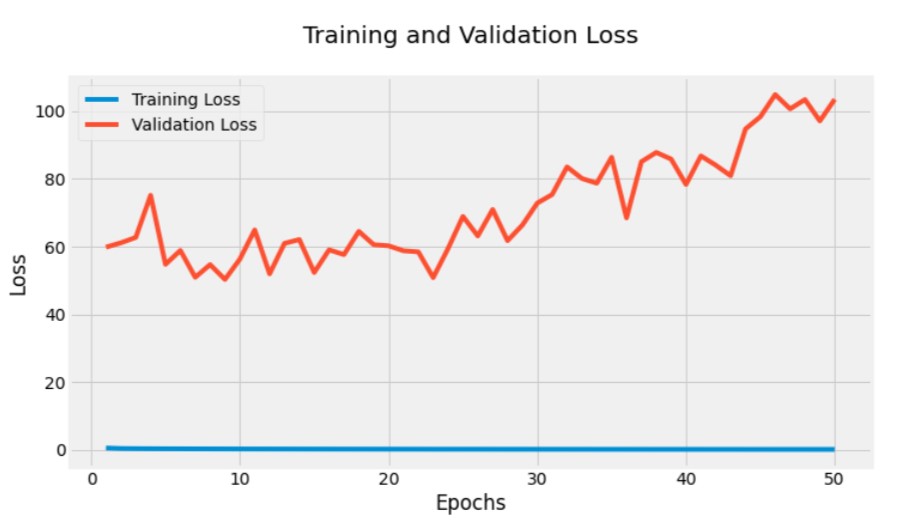
(14) Visualizing Training And Validation Loss.
plt.figure(figsize = (12, 6))
plt.style.use('fivethirtyeight')

train_loss = model_history.history['loss']
val_loss = model_history.history['val_loss']
epoch = range(1, 51)
sns.lineplot(epoch, train_loss, label = 'Training Loss')
sns.lineplot(epoch, val_loss, label = 'Validation Loss')
plt.title('Training and Validation Loss\n')
plt.xlabel('Epochs')
plt.ylabel('Loss')
plt.legend(loc = 'best')
plt.show()
(15) Visualizing Training And Validation Accuracy
plt.figure(figsize = (12, 6))

train_loss = model_history.history['accuracy']
val_loss = model_history.history['val_accuracy']
epoch = range(1, 51)
sns.lineplot(epoch, train_loss, label = 'Training accuracy')
sns.lineplot(epoch, val_loss, label = 'Validation accuracy')
plt.title('Training and Validation Accuracy\n')
plt.xlabel('Epochs')
plt.ylabel('Accuracy')
plt.legend(loc = 'best')
plt.show()

(16) Making Prediction:
# making predictions

y_probs = model.predict(X_test)
y_preds = y_probs.argmax(axis = 1)

y_preds[:100]
(17) Confusion Matrix:
# function for confusion matrix

import itertools
from sklearn.metrics import confusion_matrix

# Our function needs a different name to sklearn's plot_confusion_matrix
def make_confusion_matrix(y_true, y_pred, classes=None, figsize=(10, 10), text_size=15):
  """Makes a labelled confusion matrix comparing predictions and ground truth labels.

  If classes is passed, confusion matrix will be labelled, if not, integer class values
  will be used.

  Args:
    y_true: Array of truth labels (must be same shape as y_pred).
    y_pred: Array of predicted labels (must be same shape as y_true).
    classes: Array of class labels (e.g. string form). If `None`, integer labels are used.
    figsize: Size of output figure (default=(10, 10)).
    text_size: Size of output figure text (default=15).

  Returns:
    A labelled confusion matrix plot comparing y_true and y_pred.

  Example usage:
    make_confusion_matrix(y_true=test_labels, # ground truth test labels
                          y_pred=y_preds, # predicted labels
                          classes=class_names, # array of class label names
                          figsize=(15, 15),
                          text_size=10)
  """
  # Create the confustion matrix
  cm = confusion_matrix(y_true, y_pred)
  cm_norm = cm.astype("float") / cm.sum(axis=1)[:, np.newaxis] # normalize it
  n_classes = cm.shape[0] # find the number of classes we're dealing with

  # Plot the figure and make it pretty
  fig, ax = plt.subplots(figsize=figsize)
  cax = ax.matshow(cm, cmap=plt.cm.Blues) # colors will represent how 'correct' a class is, darker == better
  fig.colorbar(cax)

  # Are there a list of classes?
  if classes:
    labels = classes
  else:
    labels = np.arange(cm.shape[0])

  # Label the axes
  ax.set(title="Confusion Matrix",
         xlabel="Predicted label",
         ylabel="True label",
         xticks=np.arange(n_classes), # create enough axis slots for each class
         yticks=np.arange(n_classes),
         xticklabels=labels, # axes will labeled with class names (if they exist) or ints
         yticklabels=labels)

  # Make x-axis labels appear on bottom
  ax.xaxis.set_label_position("bottom")
  ax.xaxis.tick_bottom()

  # Set the threshold for different colors
  threshold = (cm.max() + cm.min()) / 2.

  # Plot the text on each cell
  for i, j in itertools.product(range(cm.shape[0]), range(cm.shape[1])):
    plt.text(j, i, f"{cm[i, j]} ({cm_norm[i, j]*100:.1f}%)",
             horizontalalignment="center",
             color="white" if cm[i, j] > threshold else "black",
             size=text_size)
plt.style.use('seaborn-dark')
make_confusion_matrix(y_true=y_test,
y_pred=y_preds,
classes=class_names,
figsize=(15, 15),
text_size=10)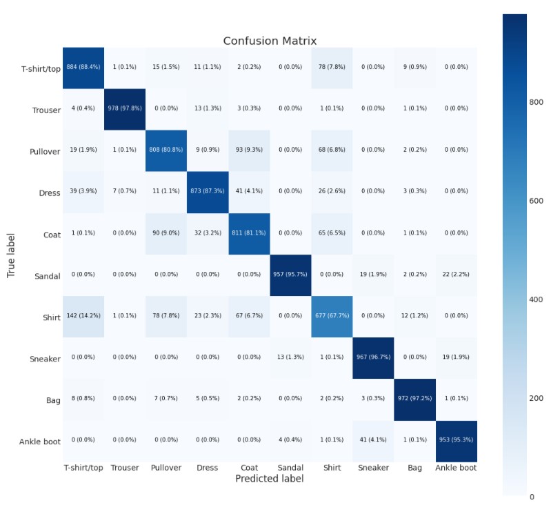
(18) Looking At Some Random Prediction
import random

# Create a function for plotting a random image along with its prediction
def plot_random_image(model, images, true_labels, classes):
  """Picks a random image, plots it and labels it with a predicted and truth label.

  Args:
    model: a trained model (trained on data similar to what's in images).
    images: a set of random images (in tensor form).
    true_labels: array of ground truth labels for images.
    classes: array of class names for images.

  Returns:
    A plot of a random image from `images` with a predicted class label from `model`
    as well as the truth class label from `true_labels`.
  """
  # Setup random integer
  i = random.randint(0, len(images))

  # Create predictions and targets
  target_image = images[i]
  pred_probs = model.predict(target_image.reshape(1, 28, 28)) # have to reshape to get into right size for model
  pred_label = classes[pred_probs.argmax()]
  true_label = classes[true_labels[i]]

  # Plot the target image
  plt.imshow(target_image, cmap=plt.cm.binary)

  # Change the color of the titles depending on if the prediction is right or wrong
  if pred_label == true_label:
    color = "green"
  else:
    color = "red"

  # Add xlabel information (prediction/true label)
  plt.xlabel("Pred: {} {:2.0f}% (True: {})".format(pred_label,
                                                   100*tf.reduce_max(pred_probs),
                                                   true_label),
             color=color) # set the color to green or red
plt.figure(figsize = (15, 12))
plotnumber = 1
for i in range(15):
if plotnumber <= 15:
ax = plt.subplot(5, 3, plotnumber)
plot_random_image(model=model,
images=X_test,
true_labels=y_test,
classes=class_names)
plotnumber += 1
plt.tight_layout()
plt.show()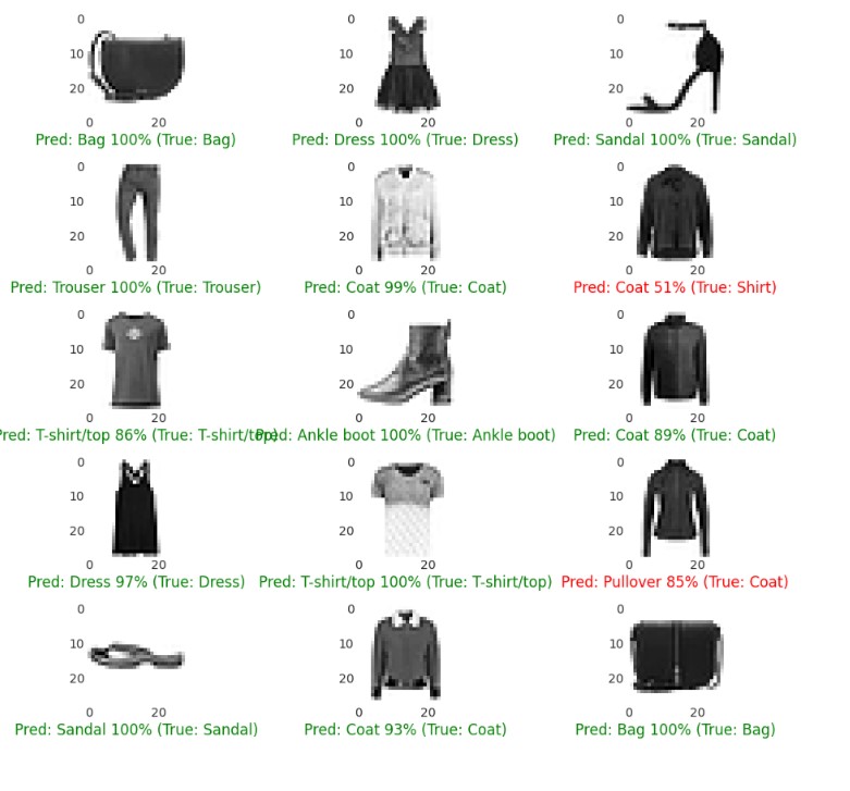
(19) Use The Model To Make Prediction
X_new = X_test[:5]
y_proba = model.predict(X_new)
y_proba.round(2)
predict_x=model.predict(X_new)
y_pred=np.argmax(predict_x,axis=1)
y_pred
np.array(class_names)[y_pred]
(19) Here, The Classification Model Actually Classified All Five Images Correctly
y_new = y_test[:5]
plt.figure(figsize=(9.2, 4.4))
for index, image in enumerate(X_new):
    plt.subplot(1, 5, index + 1)
    plt.imshow(image, cmap="binary", interpolation="nearest")
    plt.axis('off')
    plt.title(class_names[y_test[index]], fontsize=12)
plt.subplots_adjust(wspace=0.2, hspace=0.5)
plt.show()