
Transformer – Transformer Prediction
Table Of Contents:
- Prediction Setup Of Transformer.
- Step By Step Flow Of Input Sentence, “We Are Friends!”.
- Decoder Processing For Other Timestep
(1) Prediction Setup For Transformer.
Input Dataset:
- For simplicity we will take this 3 rows as input but in reality we will have thousands of rows as input.
- We will use these dataset to train our Transformer model.
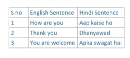
Query Sentence:
- We will pass this sentence for translation,
- Sentence = “We Are Friends !”
(2) Step By Step Flow Of Input Sentence, “We Are Friends!”.
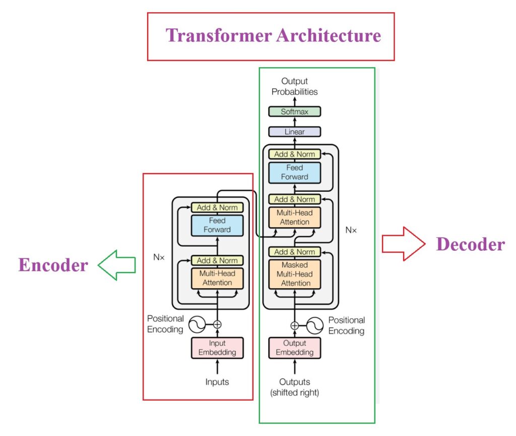
- Transformer is mainly divides into Encoder and Decoder.
- Encoder will behaves in same way at the time of training and also in prediction.
- The main difference is in Decoder part, it will behave differently at training and inference time.
- At training time i have all the output sequence in my dataset hence I can send them all at a time to decoder.
- But while prediction I will not have any information in prior what my future sequence will be. Hence we have to do sequential processing of the input.
- During training time our Decoder behaves in a Non Auto Regressive way but wile prediction it has to behave in a Autoregressive way.
- At the time of prediction we will send first <Start> token, then our decoder will know its time for prediction.
Step-1: Encoder Query Processing
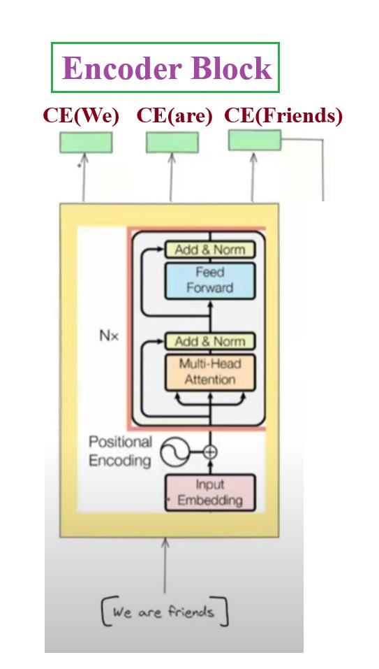
- First the query sentence “We are friends” will go to the Encoder block.
- Like this we will have 6 encoder block. The output from one encoder will go to the input to another encoder.
- Encoder block will do the processing and produce the contextual word embeddings of individual words.
- Now the decoder will have the summary of the query sentence.
Step-2: Decoder Query Processing
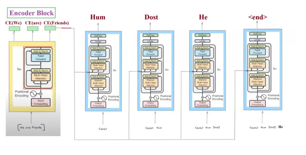
- Here you can notice that we have only one encoder that will handle all the 3 words “Hum Dost He” at a time. This shows it has Non Auto Regressive in nature.
- But we can see that we have 4 Decoder working for different time steps to handle the output. This shows it is Autoregressive in nature.
End To End Flow Of The Decoder Architecture:
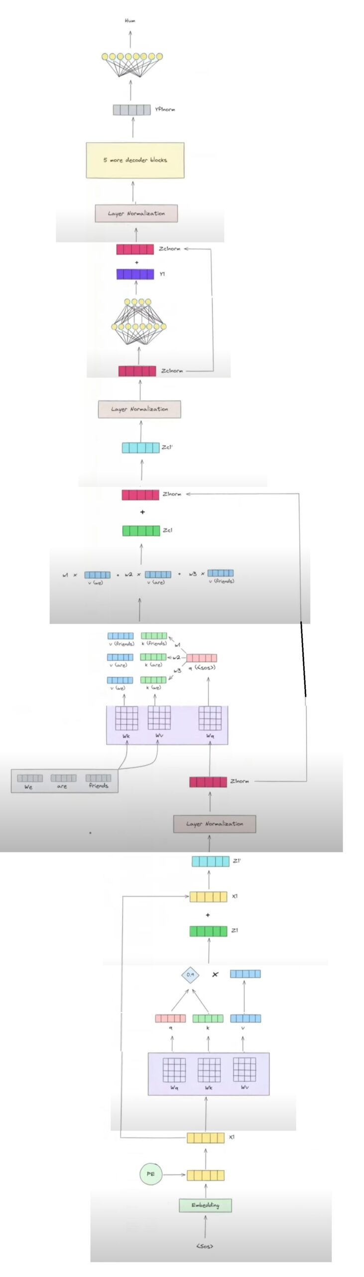
Understanding Stage -1:
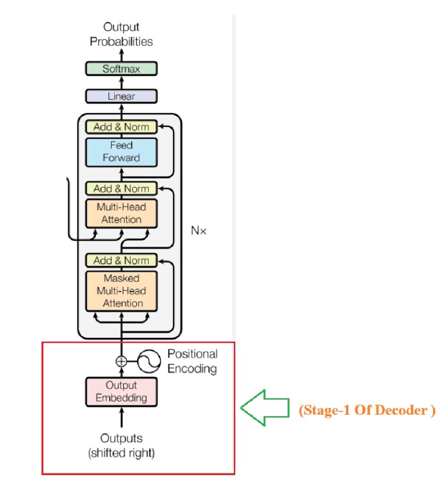
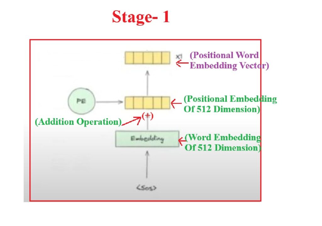
- Step-1: To start the decoding processing we have to send <Start> as the input token to the Decoder.
- Step-2: This is a English word the machine can’t understand hence we have to convert into embedding vector. Let’s pass it to the Embedding layer. It will produce 512 dimension embedding vector.
- Step-3: Generate the positional embedding vector of the input word <SOS>.
- Step-4: Add this positional embedding with the word embedding to form a new vector called ‘x1’.
- Step-5: Finally ‘X1’ will go to the Decoder as input.
Understanding Stage -2:

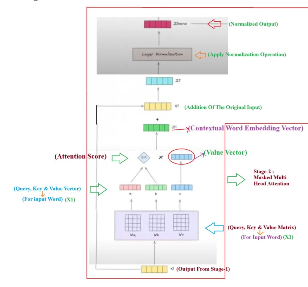
Step-1: Masked Multi Head Attention
- Step-1: You will feed output from stage -1 which is X1 to the Decoder as input.
- Step-2: First operation is Masked Multi Head Attention ,
- Step-3: Next thing is we have to generate the Query(Wq), Key(Wk) and Value(Wv) matrix from training.
- Step-4: We will do dot product of X1 with Wq, Wk and Wv to get the Query , Key and Value vector for the word <SOS>.
- Step-5: We will do the dot product of Query and Key vector to get the attention score as a scalar quantity (0.9). This 0.9 represents the similarity of <SOS> word with itself.
- Step-6: We will multiply this scalar value with the Value vector to get the contextual embedding vector of the token <SOS>.
Step-2: Addition & Normalization
- Step-1: The next step here is Add & Normalized.
- Step-2: We will add our original input vector (X1) with the Normalized vector (Z1). to retain some originality in the output vector. The output vector will be (Z1′).
- Step-3: Now we will normalize our output vector (Z1′) to stabilize our prediction process.
- Step-4: Finally we will get the (Znorm) vector as an output.
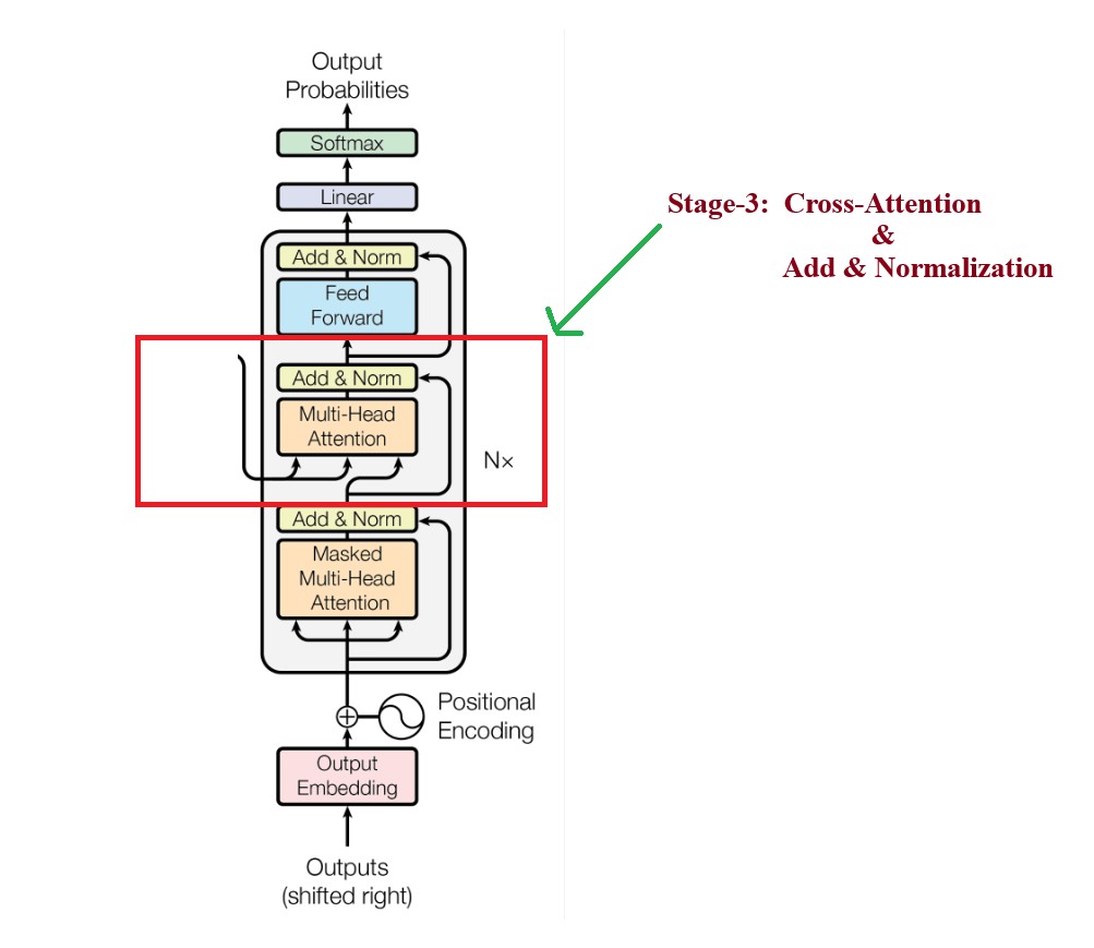
Understanding Stage -3:
- Now we will understand the Cross Attention & Add & Normalization layer.
- We will now find out the similarity between the <SOS> with the encoder input sentence individual words “We”, “are”, “friends”.
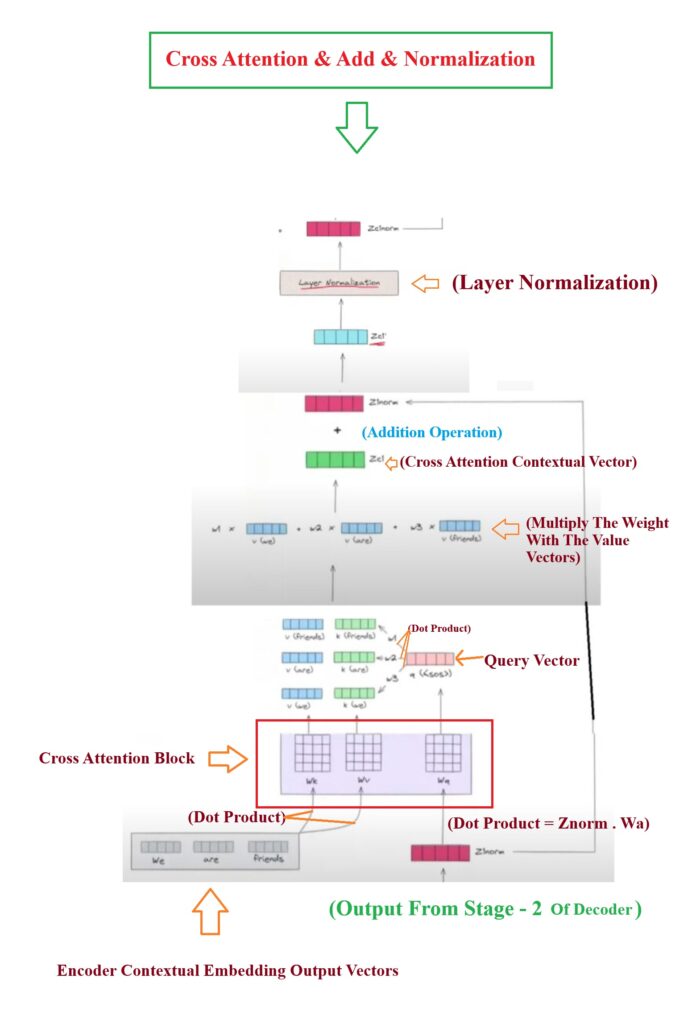
- Step-1: We will take output from Stage-2 which is Znorm and pass it to the Cross Attention Block.
- Stage-2: In Cross Attention block we will have Wk, Wv and Wq vector. These vectors we will get from training process.
- Step-3: Generally what we go we generate Query, Key and Value vectors from a single input word which in our case should be <SOS>, but in Cross attention mechanism we will use two different inputs. One is from decoder output and another is from encoder output.
- Step-4: Now we will do dot product of decoder output Znorm with the Wq (Query Matrix) and as a result we will get the Query Vector.
- Step-5: Now we will do the dot product of the Encoder output “We” , “are”, “fine” with the Wk(Key Matrix) and Wv(Value Matrix).
- Step-6: Each word of the Encoder output “We” , “are”, “fine” will get multiplied with both (Wk and Wq) matrix. “We” will get multiplied with Wk and Wv matrix and will result Key(We) and Value(We) vector.
- Step-7: Similarly we will multiply “are” vector with with Wk and Wv matrix and will result Key(are) and Value(are) vector.
- Step-8: Now for each word we have Query , Key and the Value vector. We will do the dot product of Query with the Key vector to get the attention score.
- Step-9: Perform dot product of Query vector Q<SOS> with the encoders Key vectors of each word. Q(<SOS>). K(We) = W3, Q(<SOS>). K(are) = W2, Q(<SOS>). K(friends) = W1. Now we Got weights (W1, W2 ,W3) as SCALAR VALUES.
- Step-10: Now we will multiply the weights (W1, W2 ,W3) with the Value vectors (V(We), V(are), V(friends)) for each words of the Encoder output.
- Step-11: As an output we will get the Cross Attention contextual vector.
- Step-12: Now we will do the Addition operation of the input to this stage-3 which is Znorm with the Cross Attention output.
Understanding Stage -4:
- Now we will understand the Feed Forward layer and the same Add & Norm layer.
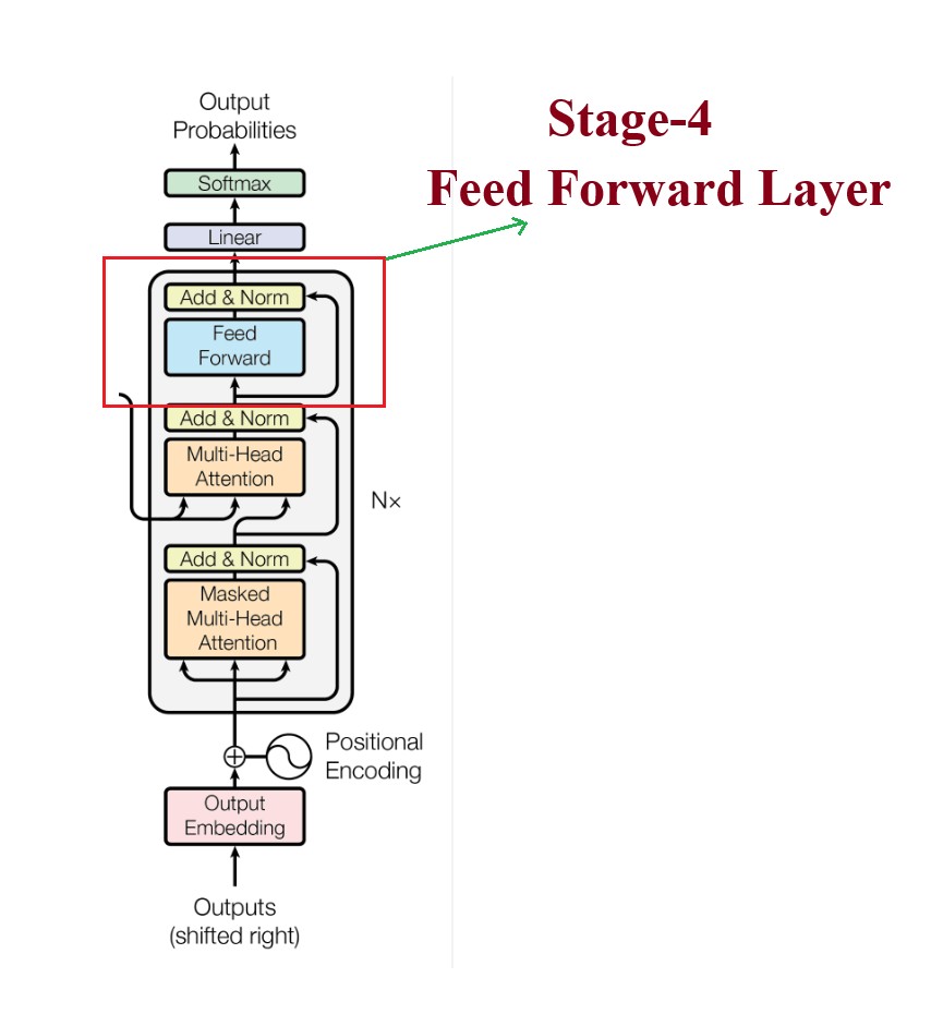
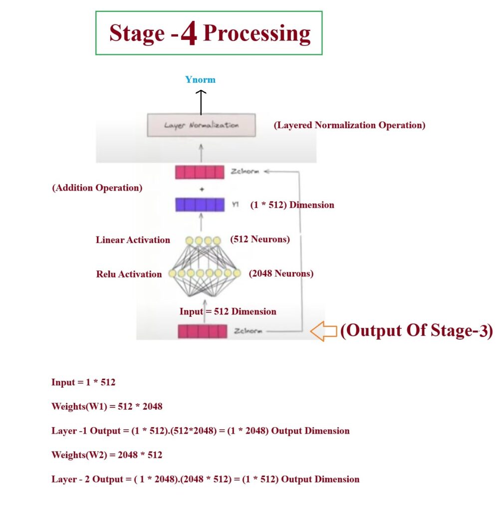
- Feed forward neural network will add some non linearith to the embedding vector.
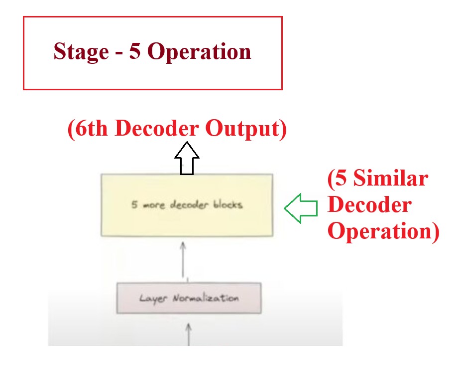
Understanding Stage -5:
- Pass the result of 1st decoder to the rest of 5 decoder sequentially fashion.
Understanding Stage -6:
- Now the final step is to make the prediction, for this we will use the Linear layer and the softmax layer.
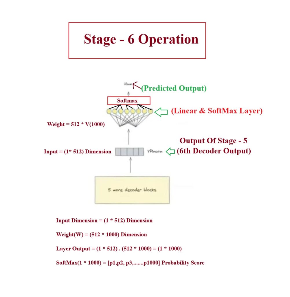
- The number of neurons in the linear layer will be the unique number of vocabulary in your Hindi sentence in your dataset.
- If unique words = 1000, V = 1000 number of neurons.
- Now input to this Linear layer will be of dimension = (1 * 512)
- Number of weights of the linear layer = (512 * 1000)
- We will do the dot product = (1 * 512) . (512 * 1000) = (1 * 1000) as an output.
- this (1 * 1000) vector will have any range of values.
- These individual values represents each unique words in the vocabulary.
- Now we will normalize this (1 * 1000) vector by passing it into the Softmax layer.
- The node with maximum probability will be considered as out output token.
(3) Decoder Processing For Other Timestep
- Output from the 1st timestep “Hum” with the <SOS> will be sent as the input to the 2nd Timestep.
- And similar processing will happen as we have seen above.
- One difference is qat the end to the Linear Layer we will pass only the embeddings of the “Hum” not both <SOS> and “Hum”.
- At prediction time also we will do the masking operation.