Data Cleaning Strategies
Table Of Contents:
- What Is Data Cleaning?
- Handling Missing Data.
- Handling Outliers.
- Removing Duplicate Data.
- Standardizing Column Names.
- Standardizing Data Formats
- Correct Data Types.
- Feature Selection.
- Feature Engineering.
- Addressing Class Imbalance.
- Dealing With Multicollinearity.
- Encoding Categorical Variables.
- Data Normalization & Standardization.
- Handling Text Data.
- Handling Time Series Data.
- Saving the Cleaned Data.
(1) What Is Data Cleaning?
- In simple terms, data cleaning is the process of fixing or removing incorrect, incomplete, or irrelevant data from a dataset.
- It ensures that the data is accurate, consistent, and ready for analysis or use in a machine learning model.

(2) Handling Missing Data.
What Is Missing Data?
- Missing data refers to the absence of a value or information for one or more variables in a dataset.
- This is common in datasets across various domains such as healthcare, finance, or surveys, where not all data points are recorded or observed.
- Missing data can arise due to various reasons like non-response in surveys, equipment malfunctions, data corruption, or manual entry errors.

Missing Value Treatment.
(1) Removing Missing Data(Row or Column Deletion)
Row Deletion: Remove rows that contain missing data.
- When to use: If only a small number of rows are affected, and removing them won’t impact the analysis significantly.
- Caution: If too many rows have missing values, this can lead to data loss and bias.
Column Deletion: Remove entire columns that contain missing values.
- When to use: If a column has too many missing values and doesn’t add much value to your analysis.
When To Use?
- When the dataset is large and only a small fraction of data is missing, or if the rows/columns with missing values are not crucial for analysis.
Drawbacks
- Can lead to significant data loss if many values are missing.
Example: Row Deletion
import pandas as pd

# Sample DataFrame
data = {'A': [1, 2, None, 4],
        'B': [None, 2, 3, 4],
        'C': [1, 2, 3, 4]}
df = pd.DataFrame(data)

df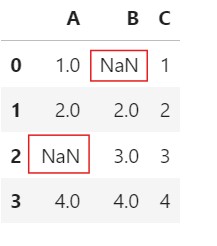
# Drop rows with any missing values
df_cleaned = df.dropna(axis=0)
df_cleaned
Example: Column Deletion
# Drop rows with any missing values
df_cleaned = df.dropna(axis=1)
df_cleaned
(2) Mean/Median/Mode Imputation
- Mean Imputation: Replace missing values with the mean of the column.
- Median Imputation: Replace missing values with the median of the column.
- Mode Imputation: Replace missing values with the mode (most frequent value) of the column.
When To Use?
- For numerical data where the values are distributed normally or uniformly.
Drawbacks
- Can introduce bias if the data has outliers or is not normally distributed.
Example:
import pandas as pd

# Sample DataFrame
data = {'A': [1, 2, None, 4],
        'B': [None, 2, 3, 4]}
df = pd.DataFrame(data)

df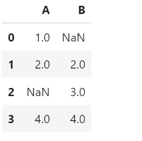
Mean Imputation:
- Filling every Null values with the Mean of the column ‘A’.
df.fillna(df['A'].mean(), inplace = True)
df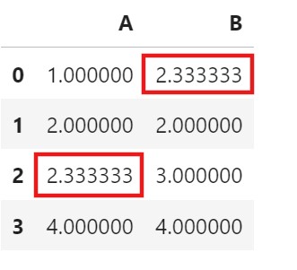
- Filling every Null values with the individual Mean of the columns.
df['A'] = df['A'].fillna(df['A'].mean())
df['B'] = df['B'].fillna(df['B'].mean())
df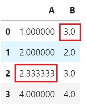
Median Imputation:
- Filling every Null values with the Median of the column ‘A’.
df.fillna(df['A'].median(), inplace = True)
df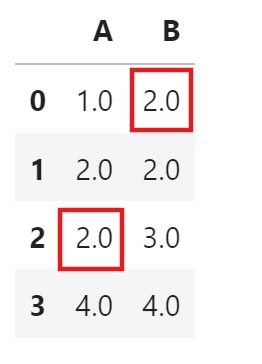
- Filling every Null values with the individual Median of the columns.
df['A'] = df['A'].fillna(df['A'].median())
df['B'] = df['B'].fillna(df['B'].median())
df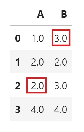
Mode Imputation:
- Filling every Null values with the Mode of the column ‘A’.
df.fillna(df['A'].mode()[0], inplace = True)
df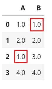
df['A'] = df['A'].fillna(df['A'].mode()[0])
df['B'] = df['B'].fillna(df['B'].mode()[0])
df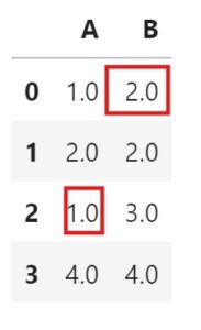
(3) Forward/Backword Fill
- Propagate the next or previous values in a column.
Forward Filling:
- Fills missing values with the last observed (previous) value.
- Useful for time-series data where previous data points are good estimates of missing ones.
- This method is useful when the data is expected to stay constant or stable over short intervals.
- For example, if values in a column are
[10, NaN, NaN, 20], forward fill would change it to[10, 10, 10, 20].
When To Use?
- In time series or sequential data where previous values provide a reasonable estimate for missing values.
Drawbacks
- Not suitable if the missing data represents a major change in the pattern or event.
Example:
import pandas as pd

# Sample DataFrame
data = {'A': [1, 2, None, 4],
        'B': [None, 2, 3, 4]}
df = pd.DataFrame(data)

df
df.fillna(method='ffill', inplace=True)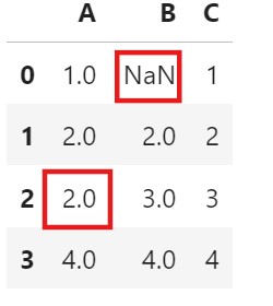
- Here, you can see that the ‘NaN’ value has not been replaced for column ‘B’.
- Because we have used the forward fill method, before the ‘NaN’ value, we do not have any value presented.
df['A'] = df['A'].fillna(method = 'ffill')Backword Filling:
- Fills missing values with the next known value.
- This method is useful when there is a delayed effect in the data, where future values can be representative of the missing ones.
- A delayed effect in data refers to situations where the impact of an event or condition is not immediately visible in the data but appears after some time.
- When patients start a new treatment, the effects might not be visible in health indicators immediately.
- Using the previous example
[10, NaN, NaN, 20], backward fill would change it to[10, 20, 20, 20].
When To Use?
- In cases where the next known value can provide a suitable estimate, often due to delayed effects in data.
Drawbacks
- May not work well if missing values are early in the sequence or if they represent unique events.
Example:
import pandas as pd

# Sample DataFrame
data = {'A': [1, 2, None, 4],
        'B': [None, 2, 3, 4]}
df = pd.DataFrame(data)

df
df.fillna(method = 'bfill', inplace=True)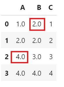
df['B'] = df['B'].fillna(method = 'bfill')
(4) Interpolate Missing Values
- Interpolation is a technique used to estimate or “fill in” missing values in a dataset by using the values of surrounding data points.
- In other words, it generates a smooth transition between known values by estimating the unknown values in between.
- This is especially useful in time series or continuous numerical data where missing points can disrupt trends or patterns.
Assumptions Off Interpolation:
- Interpolation assumes that data points near each other are likely to follow a consistent trend or pattern.
- By using known data points before and after a missing value, we can estimate the missing value based on this pattern.
Linear Interpolation:
- How it works: Fills in missing values by drawing a straight line between two known data points. The missing value is estimated based on its position between these points.
- Example: If you have data points at (1, 10) and (3, 30) with a missing value at (2, ?), linear interpolation will calculate the value at (2) as 20 because it’s halfway between 10 and 30.
- Use case: Simple, ideal for data that follows a roughly linear trend over short gaps.
Example:
import pandas as pd
data['column'] = data['column'].interpolate(method = 'linear')
Polynomial Interpolation:
- How it works: Uses a polynomial equation to fit the known data points and estimates missing values based on the curve.
- Example: Given points at (1, 2), (2, ?), and (3, 10), quadratic interpolation might estimate the missing value at (2) as 5 by fitting a parabola through the points.
- Use case: Useful for non-linear trends, such as exponential growth or curved patterns.
Example:
import pandas as pd
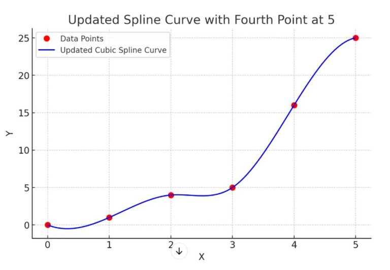
data['column'] = data['column'].interpolate(method='polynomial', order=2)Spline Interpolation:
- How it works: Fits piecewise polynomials (usually cubic) to the data, ensuring smoothness at the joins.
- Example: Given points at (1,2)(1, 2)(1,2), (2,?)(2, ?)(2,?), and (3,10)(3, 10)(3,10), cubic spline interpolation might estimate the missing value at (2)(2)(2) as 6.56.56.5 by fitting piecewise cubic polynomials through the points while ensuring smoothness at the joins.
- Use case: Ideal for smooth, continuous datasets with non-linear trends.
Example:
import pandas as pd
df['column'] = df['column'].interpolate(method='spline', order=3)
What Is Spline Curve?
- A spline is a mathematical function used to create a smooth curve through a series of data points.
- Instead of fitting a single global polynomial to the entire dataset, splines use piecewise polynomials, which are joined together at specific points called knots.
- These pieces are designed to ensure smoothness and continuity across the entire curve.
Key Characteristics Of Spline Curve.
- Piecewise Polynomial: The curve is defined as separate polynomial segments between knots.
- Smoothness: Splines ensure that the curve is smooth by maintaining continuity in the function and its derivatives (e.g., slope) at the knots.
- Flexibility: Splines can model complex, non-linear relationships without the overfitting issues of high-degree polynomials.
- Types of Splines:
- Linear Spline: A piecewise linear function, creating straight-line segments.
- Quadratic Spline: Uses quadratic polynomials for each segment.
- Cubic Spline: Uses cubic polynomials, the most common type, as it balances smoothness and computational efficiency.
Examples Of Spline Curve.
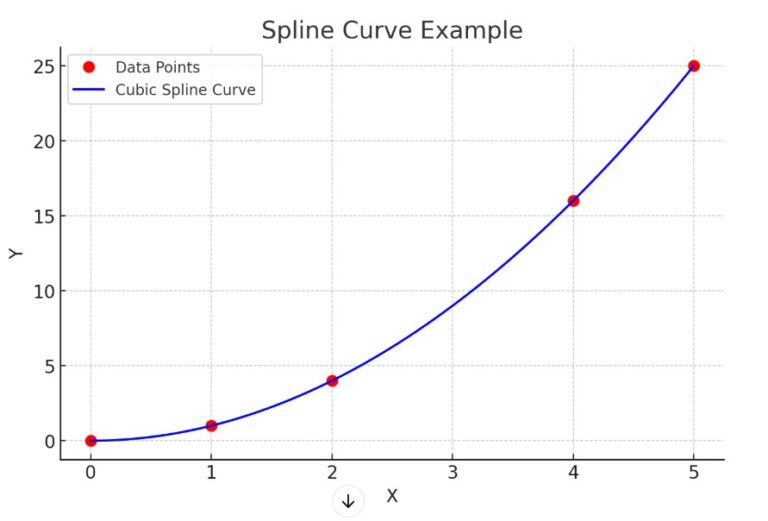
- what if in the above image the fourth data point is at value = 5 , how the spline curve looks like