Regularization In Machine Learning
Table Of Contents:
- What Is Regularization?
- Types Of Regularization Techniques.
- L1 Regularization (Lasso Regularization).
- L2 Regularization (Ridge Regularization).
- Elastic Net Regularization.
Why It Is Called Penalty?
What Does The Penalty Do
Comparison Of L1 and L2 Penalty
How to Choose the Regularization Type?
Effect of Regularization Parameter (𝜆)
Can We Apply Regularization To All The Machine Learning Models ?
(1) What Is Regularization?
- We need a regulator for our model to have control of the learning, we can have control to avoid overfitting of the model.
- Regularization in machine learning is a technique used to prevent overfitting and improve the generalization performance of a model.
- Overfitting occurs when a model learns to fit the training data too closely, capturing noise or irrelevant patterns that do not generalize well to new, unseen data.
- Regularization introduces additional constraints or penalties to the learning process to prevent the model from becoming too complex or sensitive to the training data.
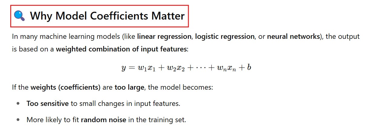
- Regularization is a technique used in machine learning to prevent overfitting by adding a penalty term to the loss function.
- It discourages the model from learning overly complex patterns that may not generalize well to unseen data.
- Regularization achieves this by controlling the magnitude of the model’s coefficients, effectively simplifying the model.

Why It Is Called Penalty?
- The penalty increases the total loss value if the coefficients are large.
- This forces the optimization algorithm to find solutions where coefficients are smaller, or in the case of L1, where some are exactly zero.
(2) Why We Need Regularization?
Overfitting:
- A model with too many features or high complexity might perform exceptionally well on the training data but poorly on the test data. This is overfitting.
- Regularization prevents the model from fitting noise in the data.
Feature Selection:
- Regularization can automatically reduce the importance of irrelevant or less relevant features by shrinking their coefficients.
(3) Types Of Regularization Technique.
- There are two common types of regularization techniques:
- L1 Regularization (Lasso Regularization).
- L2 Regularization (Ridge Regularization).
- Elastic Net Regularization.
(4) L1 Regularization
- LASSO(Least Absolute Shrinkage and Selection Operator).
- In L1 regularization, the model’s cost function is augmented with the sum of the absolute values of the model’s coefficients, multiplied by a regularization parameter (lambda).
- This encourages the model to shrink less important features’ coefficients to zero, effectively performing feature selection and promoting sparsity in the model.
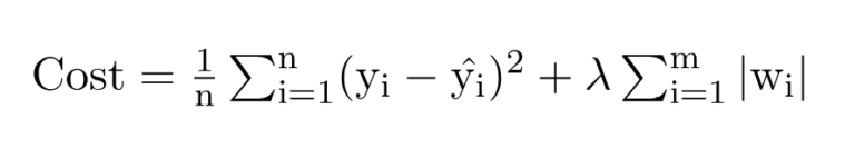
where,
- m – Number of Features
- n – Number of Examples
- w – Coefficients of Variables
- y_i – Actual Target Value
- y_i(hat) – Predicted Target Value
Limitations Of L1 Regularization:
Feature Selection Bias: L1 regularization tends to favour sparse solutions by driving some feature coefficients to exactly zero. While this can be advantageous for feature selection and model interpretability, it may also lead to a bias in feature selection. L1 regularization tends to favor one feature over another when they are highly correlated, leading to instability or arbitrary feature selection.
Lack of Stability: L1 regularization can be sensitive to small changes in the input data. This sensitivity can cause instability in feature selection, resulting in different subsets of features being selected for slightly different training sets. As a result, the model’s performance may vary significantly depending on the specific training data.
Limited Shrinkage: L1 regularization does not effectively shrink the coefficients of correlated features together. Each feature is penalized independently, leading to a lack of shrinkage for groups of correlated features. This can be problematic when dealing with datasets where many features are highly correlated, as L1 regularization may not effectively handle their collective impact.
Inconsistent Solutions: When multiple features are highly correlated, L1 regularization may produce inconsistent solutions. Small changes in the data or the optimization process can lead to different subsets of features being selected, resulting in different models and predictions.
Sensitivity to Scaling: L1 regularization is sensitive to the scale of features. Features with larger magnitudes can have a larger impact on the regularization term, potentially dominating the model’s coefficients. It is often necessary to standardize or normalize the features before applying L1 regularization to ensure fair treatment of all features.
Conclusion:
- Despite these limitations, L1 regularization remains a valuable technique for feature selection, sparsity, and interpretability.
- However, it is important to be aware of these limitations and consider alternative regularization methods, such as L2 regularization or Elastic Net, when dealing with highly correlated features or when stability and consistent solutions are critical.
(5) L2 Regularization
- In L2 regularization, the model’s cost function is augmented with the sum of the squared values of the model’s coefficients, multiplied by a regularization parameter (lambda).
- This encourages the model to distribute the impact of feature weights more evenly and reduces the impact of individual features, preventing them from dominating the model’s predictions.
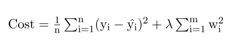
where,
- m – Number of Features
- n – Number of Examples
- w – Coefficients of Variables
- y_i – Actual Target Value
- y_i(hat) – Predicted Target Value
Limitations Of L2 Regularization:
- Inability to Perform Feature Selection: Unlike L1 regularization, L2 regularization does not drive coefficients exactly to zero. It only shrinks the coefficients towards zero without eliminating any features entirely. Consequently, L2 regularization does not inherently perform feature selection, which means all features contribute to the model, albeit with reduced magnitudes.
- Limited Ability to Handle Irrelevant Features: L2 regularization can reduce the impact of irrelevant features by shrinking their coefficients, but it does not completely eliminate their influence. In cases where there are a large number of irrelevant features, L2 regularization may not be as effective as L1 regularization in removing them from the model.
Sensitivity to Feature Scale: L2 regularization assumes that all features are on a similar scale. If the features have significantly different scales, features with larger magnitudes can dominate the regularization term and have a disproportionate impact on the model’s coefficients. It is generally recommended to normalize or standardize the features before applying L2 regularization to ensure fair regularization across all features.
Limited Ability to Handle Correlated Features: L2 regularization does not explicitly handle the issue of correlated features. Unlike L1 regularization, which tends to select one feature from a group of highly correlated features, L2 regularization does not differentiate between them and assigns similar weights to all of them. This can result in unstable and inconsistent solutions when dealing with highly correlated features.
Bias Towards Small Coefficients: L2 regularization tends to shrink all coefficients towards zero, but it does not encourage sparsity or favour solutions with a small number of non-zero coefficients. This can be a limitation when dealing with high-dimensional datasets, as L2 regularization does not inherently provide a sparse solution.
Conclusion:
- It’s important to consider these limitations when deciding whether to use L2 regularization in a particular machine-learning task.
- Depending on the specific requirements of the problem, alternative regularization techniques, such as L1 regularization or Elastic Net, may be more suitable.
(6) Elastic Net Regularization
- Elastic Net regularization is a technique in machine learning that combines both L1 (Lasso) and L2 (Ridge) regularization methods. It is used to handle situations where there are many correlated features in a dataset and helps address some limitations of using only L1 or L2 regularization individually.
where,
- m – Number of Features
- n – Number of Examples
- w – Coefficients of Variables
- y_i – Actual Target Value
- y_i(hat) – Predicted Target Value
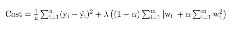
The Elastic Net regularization adds a penalty term to the model’s cost function that combines both the L1 and L2 regularization terms. The cost function is augmented with two hyperparameters: alpha and lambda.
The term alpha controls the balance between the L1 and L2 regularization. A value of 1 represents pure L1 regularization, while a value of 0 represents pure L2 regularization. Intermediate values between 0 and 1 allow for a combination of L1 and L2 regularization.
- The term lambda, similar to the regularization parameter in L1 and L2 regularization, controls the overall strength of regularization. A higher lambda value increases the amount of shrinkage applied to the model’s coefficients.
Advantages Of Elastic Net Regularization
Feature Selection: Like L1 regularization, Elastic Net can perform feature selection by driving some feature coefficients to zero. This is useful when dealing with high-dimensional datasets with many correlated features.
Handling Correlated Features: Elastic Net addresses the issue of correlated features that can cause instability in L1 regularization. The L2 regularization component helps to group correlated features together, preventing them from being excessively penalized.
Flexibility: By adjusting the alpha hyperparameter, Elastic Net allows for a flexible balance between the benefits of L1 and L2 regularization. It can capture both sparse and dense feature representations.
Conclusion:
- Elastic Net regularization is commonly used in regression problems, such as linear regression or logistic regression, where the goal is to find a suitable set of coefficients for the model. It offers a versatile regularization approach that combines the strengths of L1 and L2 regularization, providing a balance between feature selection and handling correlated features.
(7) Why It Is Called Penalty?
- The penalty increases the total loss value if the coefficients are large.
- This forces the optimization algorithm to find solutions where coefficients are smaller, or in the case of L1, where some are exactly zero.
(8) What Does The Penalty Do?
Encourages Simplicity:
- By adding the penalty to the loss function, the optimization process favors smaller coefficient values, reducing the likelihood of overfitting.
Controls Model Complexity:
- A higher penalty (lambda-λ) forces the model to shrink coefficients more aggressively, leading to simpler models.
Drives Sparsity (L1-specific):
- In L1 regularization, the penalty’s sharp corner at zero (as shown in the graph) encourages some coefficients to be exactly zero, effectively removing those features.
(9) Comparison Of L1 and L2 Penalty

This visualization compares the L1 and L2 penalties:
L1 Penalty (|β|):
- The blue line represents the L1 penalty, which has a sharp corner at β=0.
- This “sharp corner” causes the optimization process to favor exact zeros for coefficients during regularization.
L2 Penalty (β²):
- The red dashed line represents the L2 penalty, which is smooth and quadratic.
- Unlike L1, L2 shrinks coefficients gradually but does not set them to zero.
The sharp corner in the L1 penalty is what drives sparsity by encouraging some coefficients to become exactly zero, effectively selecting features in the process.
(10) How to Choose the Regularization Type?
- L1 Regularization: When you suspect many features are irrelevant and need a sparse model.
- L2 Regularization: When you want to prevent overfitting but still retain all features.
- Elastic Net: When you want the benefits of both L1 and L2.
(11) Effect of Regularization Parameter (𝜆)
- λ controls the strength of regularization:
- Small –lambda-λ: Minimal regularization, closer to the original model.
- Large – lambda-λ: Strong regularization, higher penalty, and simpler model.
(12) Effect of Regularization Parameter (𝜆)
Suppose you are building a linear regression model to predict house prices using features like size, location, and number of bedrooms. If some features (e.g., “proximity to a landmark”) are irrelevant:
- Without Regularization: The model might assign high importance to irrelevant features, leading to overfitting.
- With L1 Regularization: The model will shrink irrelevant feature coefficients to zero.
- With L2 Regularization: The model will reduce the coefficients for all features, ensuring no single feature dominates.
(13) Can We Apply Regularization To All The Machine Learning Models?
- Regularization is a powerful technique, but it is not applicable to all machine learning models.
- Its applicability depends on the type of model and its formulation. Here’s a breakdown:
Models Where Regularization Can Be Applied:
Regularization works well for models that involve optimization of a loss function. These include:
Linear Models
- Linear Regression:
- Regularized versions include Ridge (L2), Lasso (L1), and Elastic Net.
- Logistic Regression:
- Regularization prevents overfitting in classification tasks.
Generalized Linear Models
- Variants of linear models extended for different types of dependent variables, such as Poisson or binomial.
Support Vector Machines (SVM)
- Regularization controls the margin and prevents overfitting through the cost parameter C.
Neural Networks
- Regularization techniques like:
- L1 and L2 penalties on weights.
- Dropout: Randomly drops neurons during training to reduce overfitting.
- Early stopping: Halts training when performance stops improving on validation data.
Tree-Based Models with Extensions
- Gradient Boosting (e.g., XGBoost, LightGBM, CatBoost):
- Regularization terms can penalize complex trees.
- Random Forests:
- Indirect regularization via hyperparameters like the maximum depth of trees and the minimum number of samples per split.
Kernel Methods
- Methods like Gaussian Processes or Kernel Ridge Regression use regularization to control complexity.
- Linear Regression:
Models Where Regularization Does Not Directly Apply
For some models, regularization is either unnecessary or cannot be directly incorporated:
Decision Trees
- Pure decision trees (e.g., CART, ID3) do not use regularization directly because they work by recursively splitting data.
- Overfitting control is done via pruning techniques or by setting hyperparameters like:
- Maximum depth
- Minimum samples per split
K-Nearest Neighbors (KNN)
- Regularization isn’t directly applicable because KNN is non-parametric and does not involve coefficient optimization.
- Overfitting is controlled by adjusting the number of neighbors kkk or distance metrics.
Naive Bayes
- Regularization isn’t applicable because Naive Bayes uses probabilities and conditional independence assumptions, not coefficient optimization.
Clustering Algorithms
- Algorithms like K-Means and DBSCAN do not involve regularization. Overfitting control depends on:
- The number of clusters.
- Choice of distance metrics.
Ensemble Models
- Models like bagging (e.g., Random Forest) inherently reduce overfitting via averaging but do not use explicit regularization.
Why Can’t Regularization Be Applied to All Models?
- Parametric Models: Regularization works well for models with parameters optimized via a loss function (e.g., linear regression, neural networks).
- Non-Parametric Models: Models like KNN or decision trees are driven by data structure and rules, not by parameters, so regularization is not directly relevant.
- Inherent Overfitting Control: Some models like Random Forest or boosting already incorporate techniques to prevent overfitting without explicitly using regularization.
Conclusion:
- Regularization is highly effective for parametric models that optimize a loss function, but its applicability varies for other types of models.
- For non-parametric models, alternative methods (like hyperparameter tuning or pruning) serve a similar purpose of reducing overfitting.
- Always choose the appropriate technique based on the model and the data characteristics!