
Heart Failure Prediction
Table Of Contents:
- What Is The Business Use Case?
- Steps Involved In Heart Failure Prediction.
- Importing Library
- Loading Data
- Plotting Count Plot
- Examining The Correlation Matrix
- For All The Features.
- Examining Count Plot Of Age.
- Outlier Detection Plotting.
- KDE Plot.
- Data Preprocessing.
- Train Test Split.
- Model Building.
- Model Conclusion.
(1) What Is The Business Use Case?
- Cardiovascular diseases are the most common cause of death globally, taking an estimated 17.9 million lives each year, which accounts for 31% of all deaths worldwide.
- Heart failure is a common event caused by Cardiovascular diseases. It is characterized by the heart’s inability to pump an adequate blood supply to the body.
- Without sufficient blood flow, all major body functions are disrupted. Heart failure is a condition or a collection of symptoms that weaken the heart.
(2) Steps Involved In Heart Failure Prediction.
- Importing Library.
- Loading Data.
- Data Analysis.
- Data Preprocessing.
- Model Building.
- Conclusion.
(3) Importing Library
import numpy as np
import pandas as pd
import matplotlib.pyplot as plt
from sklearn import preprocessing
from sklearn.preprocessing import StandardScaler
from sklearn.model_selection import train_test_split
import seaborn as sns
from keras.layers import Dense, BatchNormalization, Dropout, LSTM
from keras.models import Sequential
from keras.utils import to_categorical
from keras import callbacks
from sklearn.metrics import precision_score, recall_score, confusion_matrix, classification_report, accuracy_score, f1_score
(4) Loading Data
data = pd.read_csv('heart_failure_clinical_records_dataset.csv')
data.head()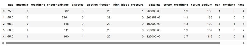
data.info()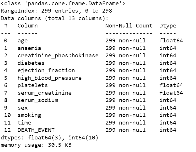
About The Data:
- age: Age of the patient
- anaemia: If the patient had the haemoglobin below the normal range
- creatinine_phosphokinase: The level of the creatine phosphokinase in the blood in mcg/L
- diabetes: If the patient was diabetic
- ejection_fraction: Ejection fraction is a measurement of how much blood the left ventricle pumps out with each contraction
- high_blood_pressure: If the patient had hypertension
- platelets: Platelet count of blood in kiloplatelets/mL
- serum_creatinine: The level of serum creatinine in the blood in mg/dL
- serum_sodium: The level of serum sodium in the blood in mEq/L
- sex: The sex of the patient
- smoking: If the patient smokes actively or ever did in past
- time: It is the time of the patient’s follow-up visit for the disease in months
- DEATH_EVENT: If the patient is deceased during the follow-up period.
(5) Plotting Count Plot
- We begin our analysis by plotting a count plot of the target attribute. A correlation matrix of the various attributes is used to examine the importance of the feature.
cols = ['red', 'blue']
sns.countplot(x = data['DEATH_EVENT'], palette = cols)
- The point to note is that there is an imbalance in the data.
(6) Examining The Correlation Matrix For All The Features.
cmap = sns.diverging_palette(275, 150,  s=40, l=65, n=9)
corrmat = data.corr()
plt.subplot(figsize = (18, 18))
sns.heatmap(corrmat, cmap = cmap, annot = True, square = True)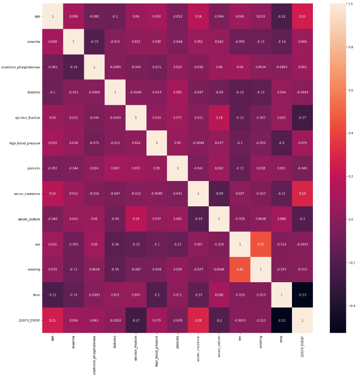
Note:
- The time of the patient’s follow-up visit for the disease is crucial as the initial diagnosis of the cardiovascular issue and treatment reduces the chances of any fatality. It holds an inverse relation.
- The ejection fraction is the second most important feature. It is quite expected as it is the efficiency of the heart.
- The age of the patient is the third most correlated feature. Clearly as the heart’s functioning declines with ageing.
(7) Examining Count Plot Of Age:
#Evauating age distrivution
plt.figure(figsize=(20,12))
Days_of_week=sns.countplot(x=data['age'],data=data, hue ="DEATH_EVENT",palette = cols)
Days_of_week.set_title("Distribution Of Age", color="#774571")
Note:
- The above diagram shows the death ratios at particular ages.
- At age 60 the non-death-to-death ratio is quite significant.
(8) Outlier Detection Plotting:
- Boxen and swarm plot of some non-binary features.
feature = ["age","creatinine_phosphokinase","ejection_fraction","platelets","serum_creatinine","serum_sodium", "time"]
for i in feature:
    plt.figure(figsize=(8,8))
    sns.swarmplot(x=data["DEATH_EVENT"], y=data[i], color="black", alpha=0.5)
    sns.boxenplot(x=data["DEATH_EVENT"], y=data[i], palette=cols)
    plt.show()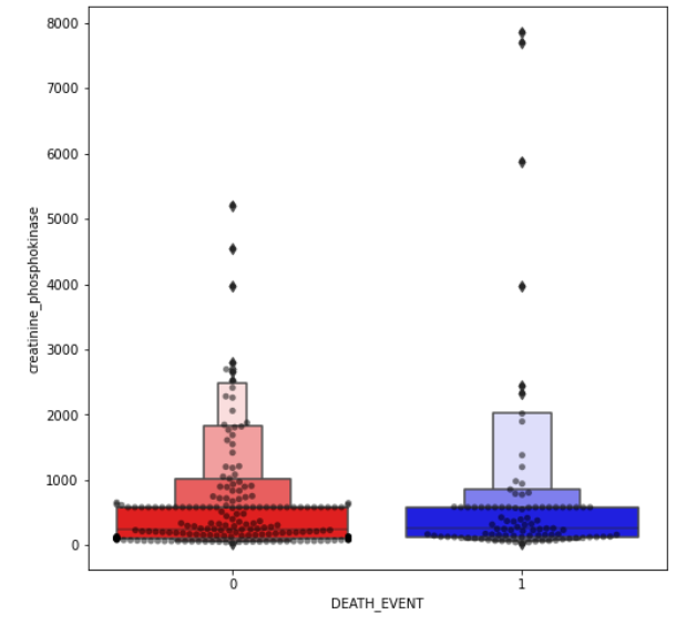


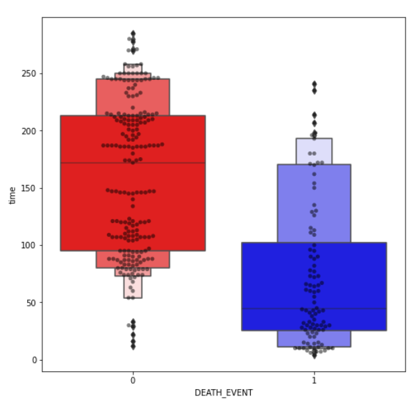
Note:
- I spotted outliers on our dataset. I didn’t remove them yet as it may lead to overfitting.
- Though we may end up with better statistics. In this case, with medical data, the outliers may be an important deciding factor.
(9) KDE Plot:
- Next, we examine the kdeplot of time and age as they both are significant features.
sns.kdeplot(x = data['time'], y = data['age'], hue = data['SEATH_EVENT'], palette = cols)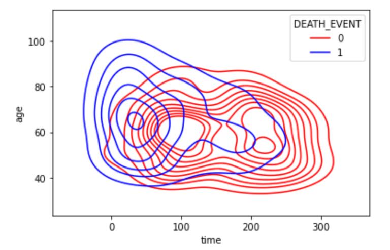
(10) Data Preprocessing:
Steps involved in Data Preprocessing
- Dropping the outliers based on data analysis
- Assigning values to features as X and target as y
- Perform the scaling of the features
- Split test and training sets
Assigning Values To Features As X And Target As y :
X = data.drop(['DEATH_EVENT'], axis = 1)
y = data['DEATH_EVENT']
Applying Standard Scalar For The Features:
col_names = list(X.columns)
s_scaler = preprocessing.StandardScaler()
X_df = s_scaler.fit_transform(X)
X_df = pd.DataFrame(data = X_df, columns = col_names)
X_df.head()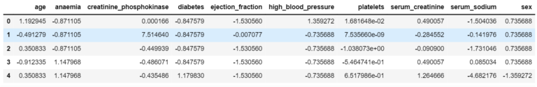
Box Plot For Scaled Features:
colours =["#774571","#b398af","#f1f1f1" ,"#afcdc7", "#6daa9f"]
plt.figure(figsize = (20,10))
sns.boxenplot(data = X_df, palette = colours)
plt.xticks(rotation = 90)
plt.show()
(11) Train Test Split:
X_train, X_test, y_train, y_test = train_test_split(X_df, y, test_size = 0.2, random_state = 2)
print('X Train: ', X_train.shape)
print('X Test: ',  X_test.shape)
print('y Train: ', X_train.shape)
print('y Test: ',  X_test.shape)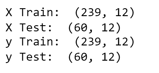
(12) Model Building:
The following steps are involved in the model building
- Initialising the ANN
- Defining by adding layers
- Compiling the ANN
- Train the ANN
Defining Early Stopping Method:
early_stopping = callbacks.EarlyStopping(
                           min_delta=0.001, # minimium amount of change to count as an improvement
                           patience=20, # how many epochs to wait before stopping
                           restore_best_weights=True
                          )
Model Initialization:
model.sequential()Adding Dense Layers:
model.add(Dense(units = 16, input_dim = 12, activation = 'relu', kernel_initializer = 'uniform'))
model.add(Dense(units = 8, kernel_initializer = 'uniform', activation = 'relu'))
model.add(Dropout(0.25))
model.add(Dense(units = 4, kernel_initializer = 'uniform', activation = 'relu'))
model.add(Dropout(0.5))
model.add(Dense(units = 1, kernel_initializer = 'uniform', activation = 'sigmoid'))
Model Compilation:
model.compile(loss = 'binary_crossentropy', optimizer = 'adam', metrics = ['accuracy'])Training The ANN Model:
history = model.fit(X_train, y_train, ebatch_size = 32, epochs = 500, callbacks = [early_stopping], validation_split = 0.2)Validation Accuracy:
val_accuracy = np.mean(history.history['val_accuracy'])
print("\n%s: %.2f%%" % ('val_accuracy', val_accuracy*100))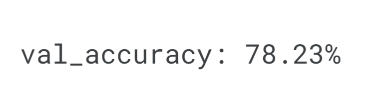
history_df = pd.DataFrame(history.history)

history_df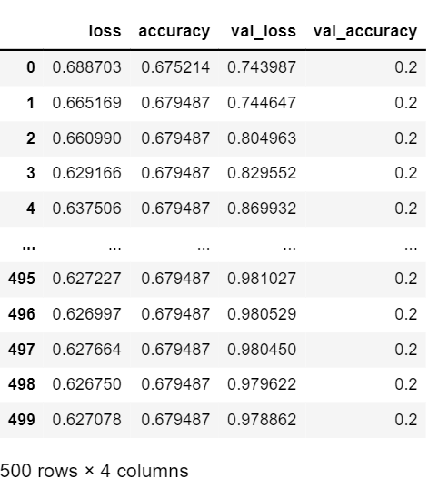
Plotting Training And Validation Loss Over Epochs:
history_df = pd.DataFrame(history.history)

plt.plot(history_df.loc[:, ['loss']], "#6daa9f", label='Training loss')
plt.plot(history_df.loc[:, ['val_loss']],"#774571", label='Validation loss')
plt.title('Training and Validation loss')
plt.xlabel('Epochs')
plt.ylabel('Loss')
plt.legend(loc="best")

plt.show()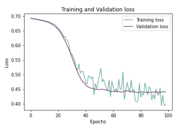
Plotting Training And Validation Accuracy Over Epochs:
history_df = pd.DataFrame(history.history)

plt.plot(history_df.loc[:, ['accuracy']], "#6daa9f", label='Training accuracy')
plt.plot(history_df.loc[:, ['val_accuracy']], "#774571", label='Validation accuracy')

plt.title('Training and Validation accuracy')
plt.xlabel('Epochs')
plt.ylabel('Accuracy')
plt.legend()
plt.show()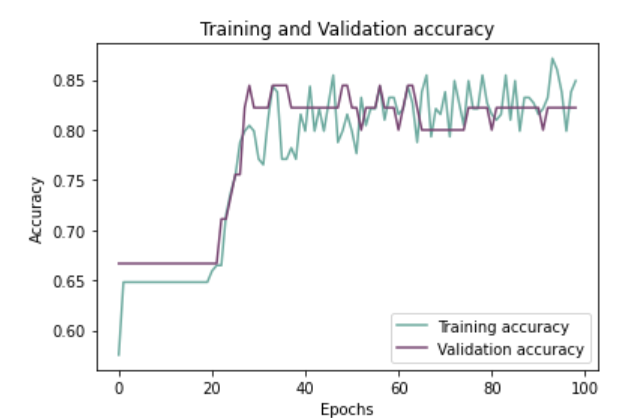
(13) Model Conclusion:
Concluding the model with:
- Testing on the test set
- Evaluating the confusion matrix
- Evaluating the classification report
Predicting The Test Set Results:
y_pred = model.predict(X_test)
y_pred = (y_pred > 0.5)
y_pred
Evaluating The Confusion Matrix:
cmap1 = sns.diverging_palette(275,150,  s=40, l=65, n=6)
plt.subplots(figsize = (12, 8))
cf_matrix = confusion_matrix(y_test, y_pred)
sns.heatmap(cf_matrix, cmap = cmap1, annot = True, annot_kws = {'size':15})
Evaluating The Classification Report:
print(classification_report(y_test, y_pred))