import pandas as pd
import seaborn as sns
import statsmodels.api as sm
from statsmodels.stats.outliers_influence import variance_inflation_factor
# Load dataset
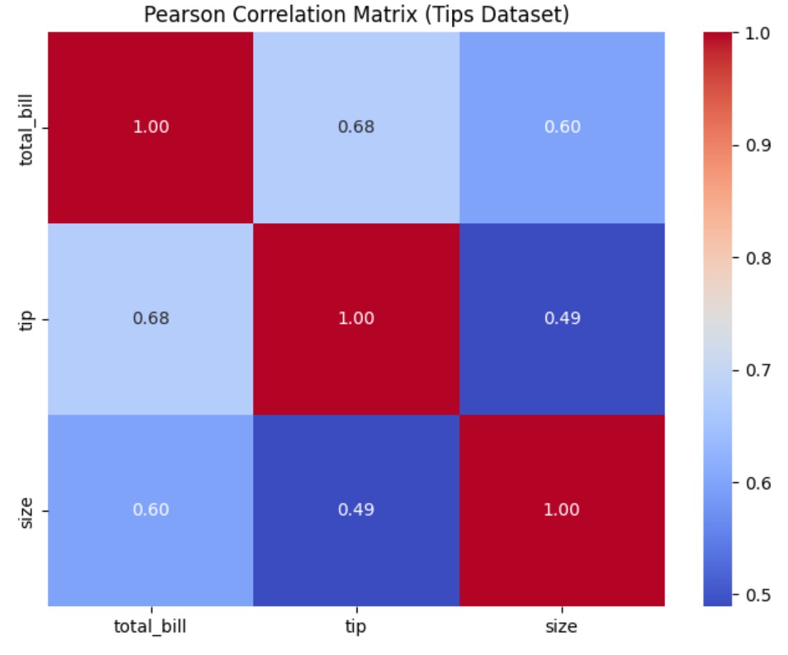
tips = sns.load_dataset('tips')
# Select relevant numerical features (exclude categorical)
df = tips[["total_bill", "tip", "size"]]
# Add a constant term for intercept
df_with_const = sm.add_constant(df)
# Calculate VIF for each feature
vif_data = pd.DataFrame()
vif_data["Feature"] = df_with_const.columns
vif_data["VIF"] = [variance_inflation_factor(df_with_const.values, i)
for i in range(df_with_const.shape[1])]
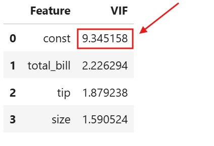
print(vif_data)
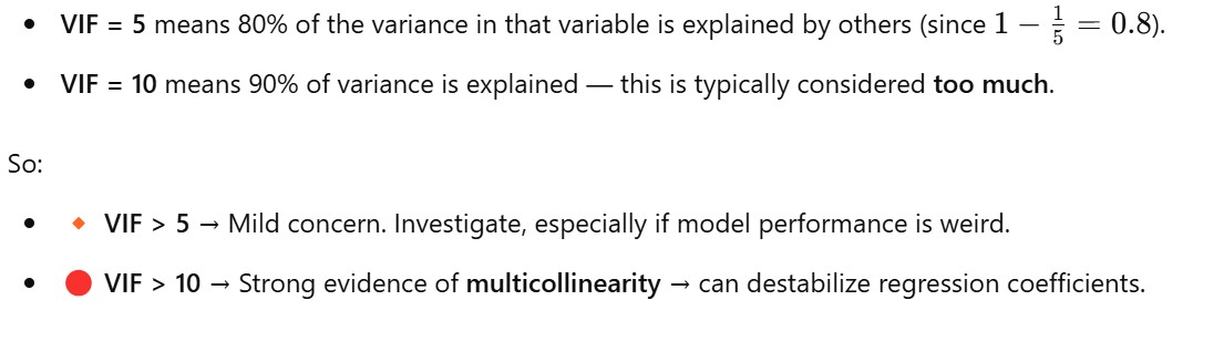
Why we use the lower limit as 5 and upper limit as 10 ?
For VIF = 5, R-Squared = 0.80, which means 80 % of the variance present in the dependent variable is explained by all the independent variable.
For VIF = 10, R-Squared = 0.90, which means 90 % of the variance present in the dependent variable is explained by all the independent variable.
Method – : Model Behavior
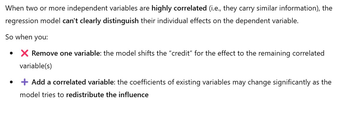
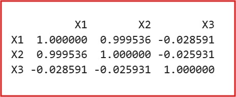
You have two features, X1 and X2, that are highly correlated. They’re both providing very similar information to the model.
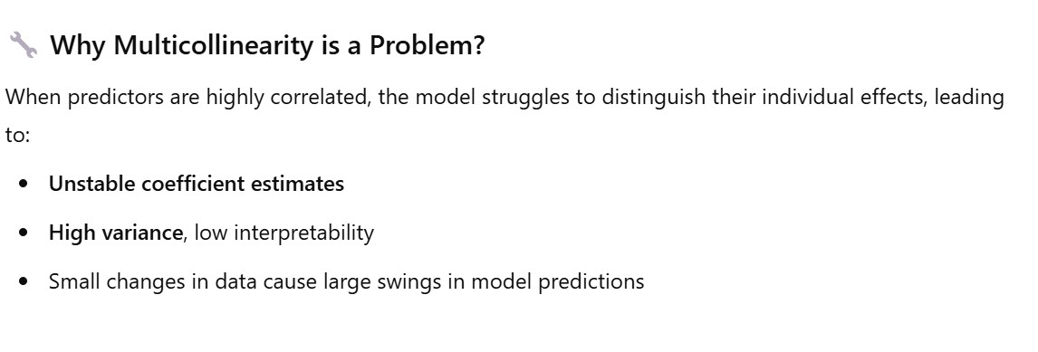
So when the model fits: It’s hard to know how much weight (coefficient) to give to X1 and X2, because changing one’s value affects the other.
This causes multicollinearity, and the model starts “splitting the credit” between them in a shaky way.
Note: After giving the unstable weights to the two variable, if you remove one variable (x2) its credit or contribution will go to other correlated variable (x1).
Hence its weight will drastically increase or decrease. With a large unit.
Question: Now the question is why the weight not got distributed to other non correlated variable ?
Answer:X1 and X2 shared a lot of overlapping info. When you remove X2, that info still exists in X1. So the model naturally adjusts the coefficient of X1 to account for that extra explanation. It’s not that the effect “jumps” to X1, but rather that the shared information already exists in X1 — so the model just leans more heavily on it.
Only the unique variance that was explained only by X2 (and not by X1) gets pushed to the residual/error term.
But if X1 and X2 are, say, 90% correlated, then removing X2 doesn’t hurt the model much — because X1 is doing almost the same job.
(2) How To Avoid Multicollinearity In The Dataset ?
Method – 1: Remove One of the Correlated Variables
Best When:Two or more variables have high correlation (Pearson’s r > 0.7 or VIF > 5/10), and you can justify removing one based on domain knowledge.
import pandas as pd
from statsmodels.api import OLS, add_constant
from statsmodels.stats.outliers_influence import variance_inflation_factor
# Sample data
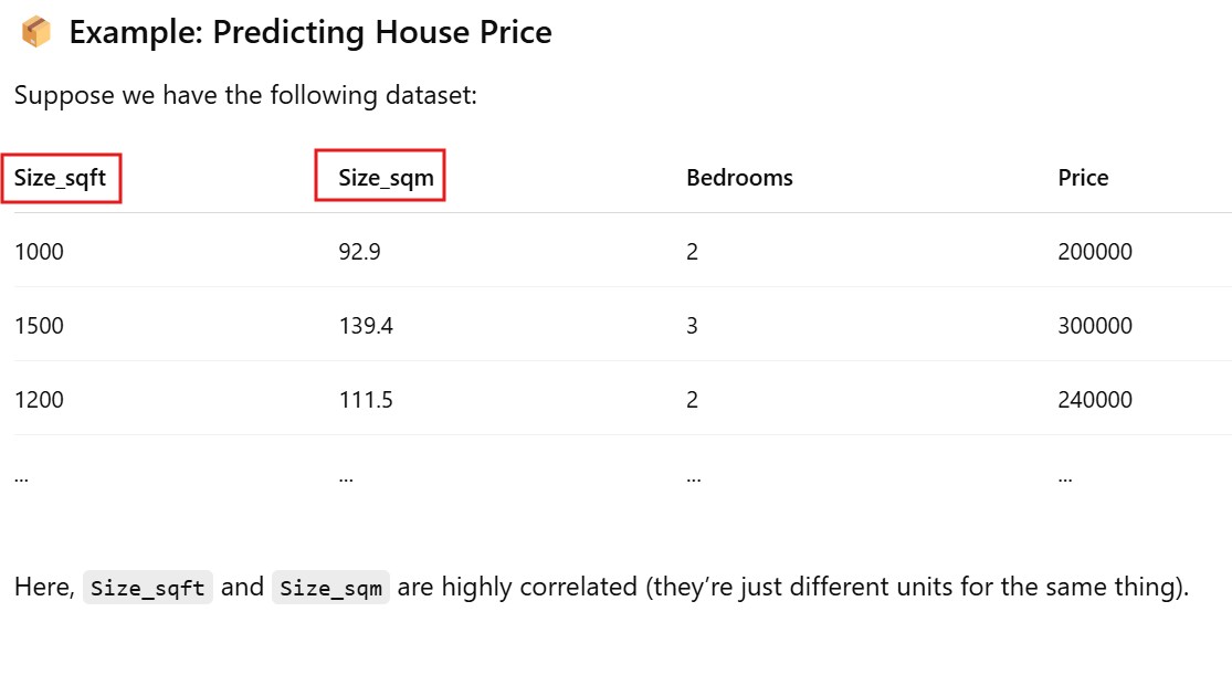
data = pd.DataFrame({
'Size_sqft': [1000, 1500, 1200, 1800, 1600],
'Size_sqm': [92.9, 139.4, 111.5, 167.2, 148.6],
'Bedrooms': [2, 3, 2, 4, 3],
'Price': [200000, 300000, 240000, 360000, 320000]
})
# Features and target
X = data[['Size_sqft', 'Size_sqm', 'Bedrooms']]
y = data['Price']
# Add constant
X_const = add_constant(X)
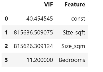
# Check VIF
vif = pd.DataFrame()
vif["VIF"] = [variance_inflation_factor(X_const.values, i) for i in range(X_const.shape[1])]
vif["Feature"] = X_const.columns
print(vif)
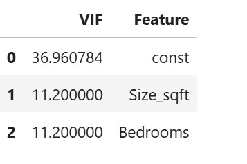
# Drop one of the correlated features
X_reduced = data[['Size_sqft', 'Bedrooms']]  # Removed 'Size_sqm'

# Refit model or calculate new VIF
X_const = add_constant(X_reduced)
vif = pd.DataFrame()
vif["VIF"] = [variance_inflation_factor(X_const.values, i) for i in range(X_const.shape[1])]
vif["Feature"] = X_const.columns
vif
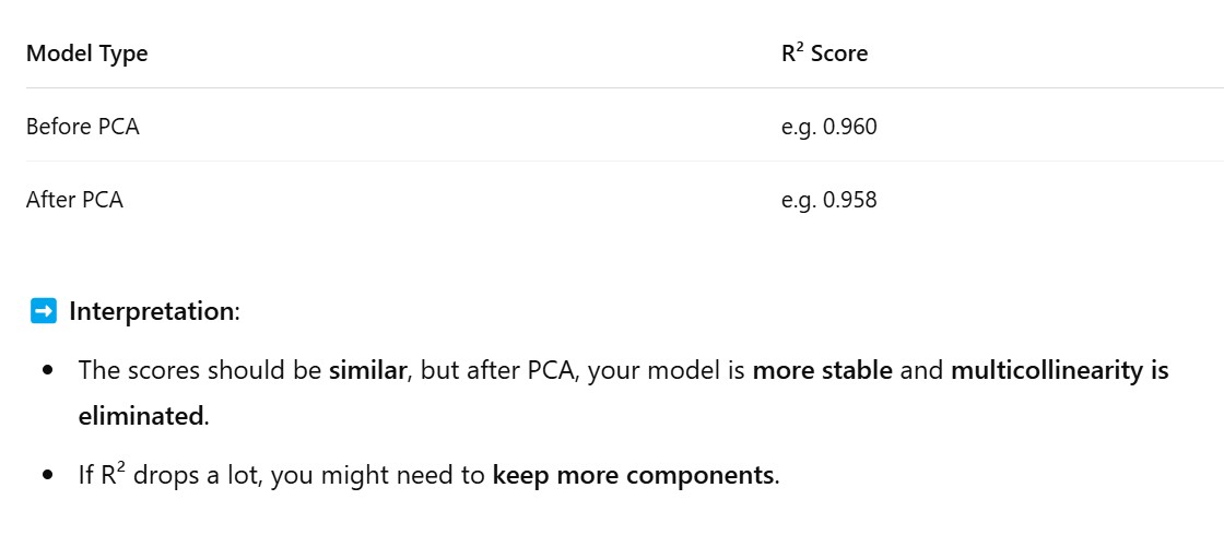
Method – 2: Use Principle Component Analysis(PCA)
Step 1: Import Libraries & Create a Dataset with Multicollinearity
import numpy as np
import pandas as pd
from sklearn.decomposition import PCA
from sklearn.preprocessing import StandardScaler
from sklearn.linear_model import LinearRegression
from sklearn.model_selection import train_test_split
# Create synthetic dataset with multicollinearity
np.random.seed(42)
X1 = np.random.rand(100) * 100
X2 = X1 + np.random.normal(0, 1, 100) # Strongly correlated with X1
X3 = np.random.rand(100) * 50
# Target variable
y = 5 + 2 * X1 + 3 * X3 + np.random.normal(0, 10, 100)
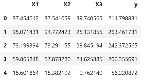
# Create DataFrame
df = pd.DataFrame({'X1': X1, 'X2': X2, 'X3': X3, 'y': y})