Linear Regression – Assumption- 1 (Linear Relationship)
Table Of Contents:
What Is Q – Q Plot ?
Example Of Q – Q Plot .
Why There Is A Straight Line In The Q – Q Plot ?
(1) What Is Q – Q Plot ?
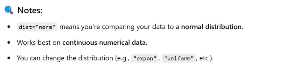
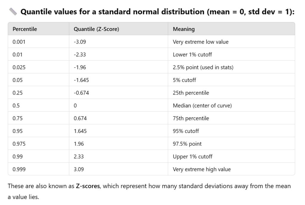
A Q–Q plot (Quantile–Quantile plot) is a probability plotthat compares the quantiles of a dataset to the quantiles of a theoretical distribution (often the normal distribution).
It helps to visually check if your data is normally distributed.
(2) When to use a Q–Q Plot ?
To assess normality (Is my data normally distributed?)
To detect skewness, outliers, or distribution mismatches.
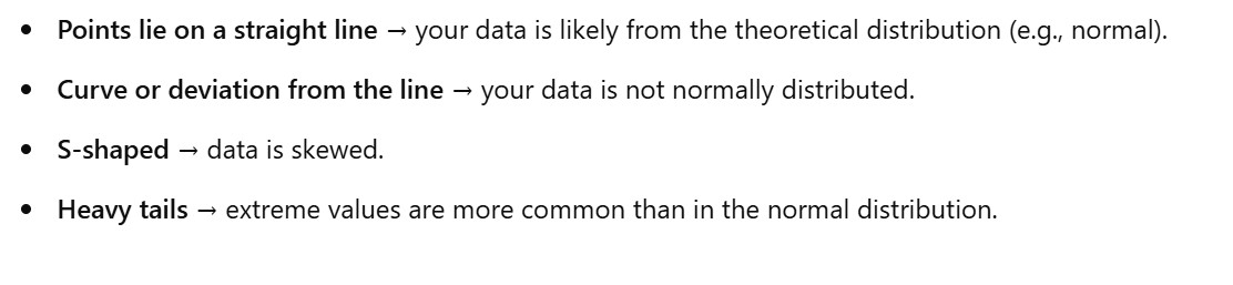
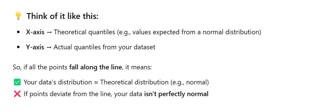
(3) Interpreting Q–Q Plot ?
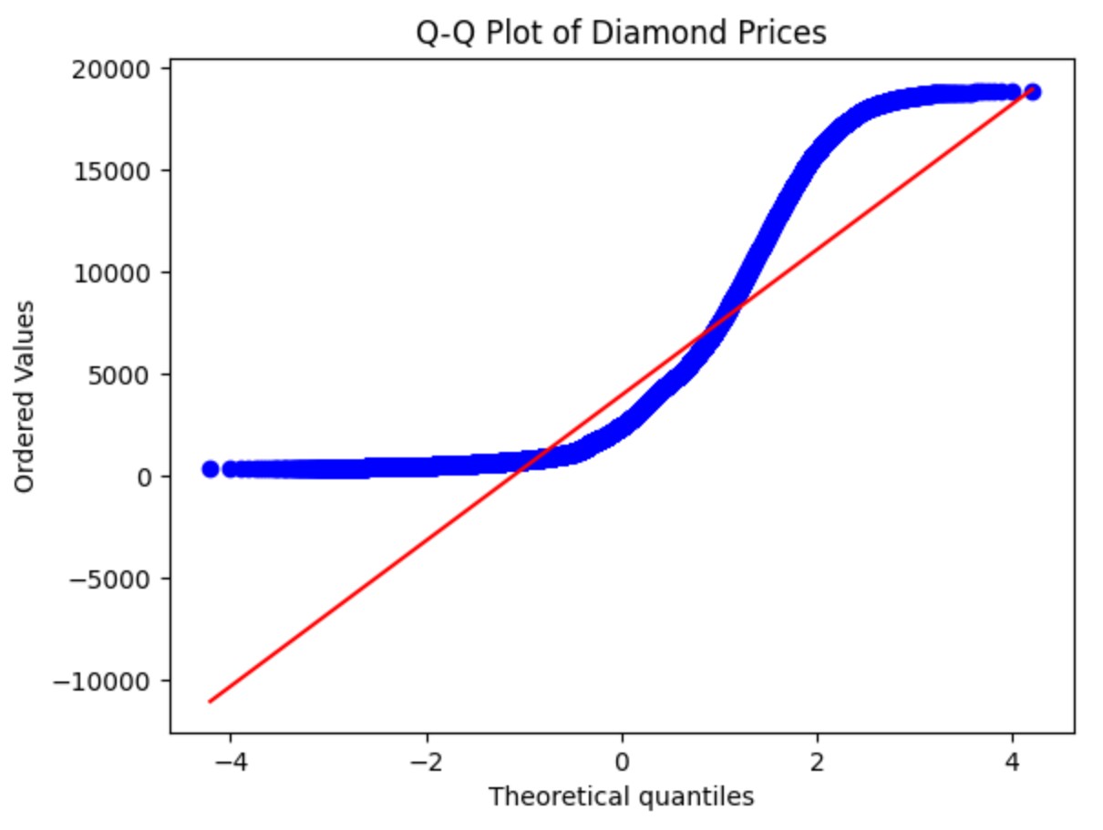
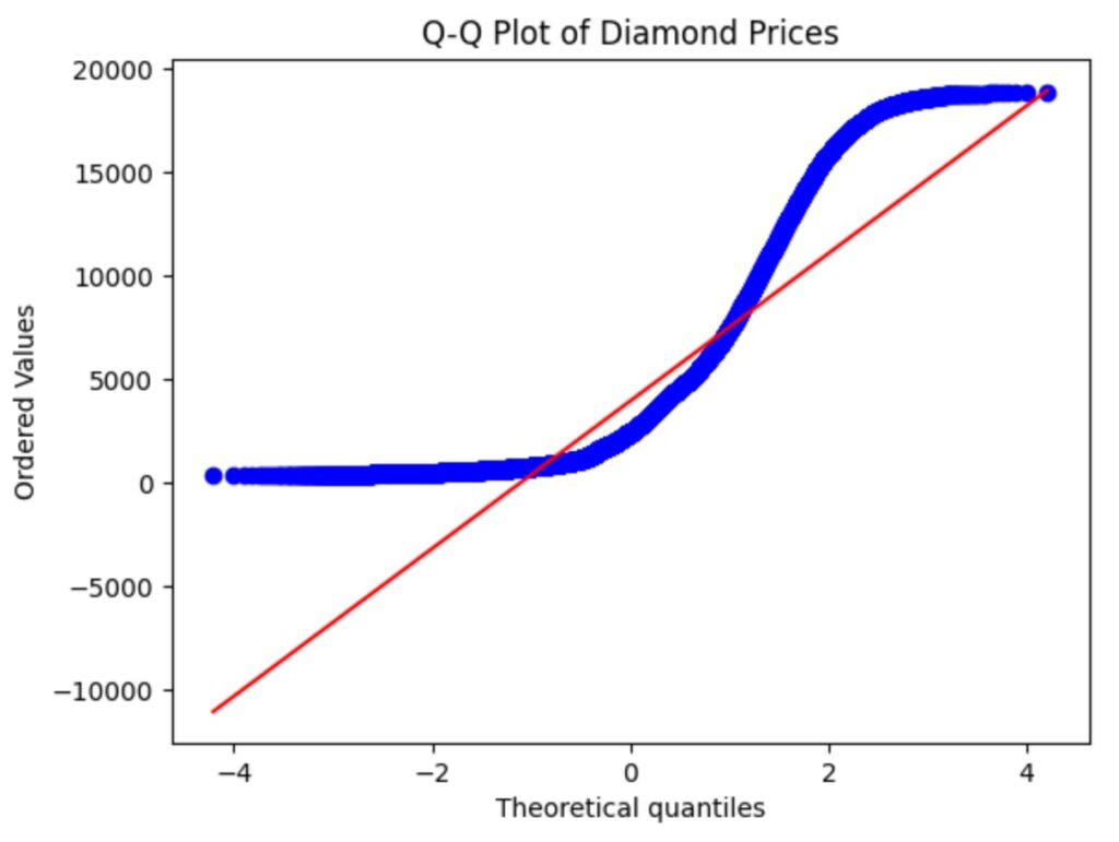
(4) Example Of Q–Q Plot ?
import seaborn as sns
import matplotlib.pyplot as plt
import scipy.stats as stats

# Load sample data
data = sns.load_dataset("diamonds")  # built-in Seaborn dataset
x = data["price"]  # taking the 'price' column

# Q-Q plot
stats.probplot(x, dist="norm", plot=plt)
plt.title("Q-Q Plot of Diamond Prices")
plt.show()
(5) Why There Is A Straight Line In Q – Q Plot ?
The straight line(also called the reference line or theoretical line) represents the ideal case — what the quantiles of your data would look like if they were perfectly following the specified theoreticaldistribution (usually the normal distribution).
The straight line is the ideal condition when your data quantile value matches with the normal distribution quantile value.