Customer Churn Prediction In Banking Sector
Table Of Contents:
- What Is The Business Use Case?
- List Of Independent Variables.
- Importing Necessary Libraries for Artificial Neural Network.
-
Importing Dataset.
- Generating Matrix of Features (X).
- Generating Dependent Variable Vector(Y).
- Encoding Categorical Variable Gender.
- Encoding Categorical Variable Country.
- Splitting Dataset into Training and
- Testing Dataset.
- Performing Feature Scaling.
- Initializing Artificial Neural Network.
- Creating Hidden Layers.
- Creating Output Layer.
- Compiling Artificial Neural Network.
- Fitting Artificial Neural Network.
- Predicting Result for Single Point Observation.
- Saving Created Neural Networks.
(1) What Is Business Use Case ?
- Business Use Cases: Customer Churn Prediction In the Banking Sector.
- Please find the high-risk customers who will close their bank accounts and discontinue with the Bank.

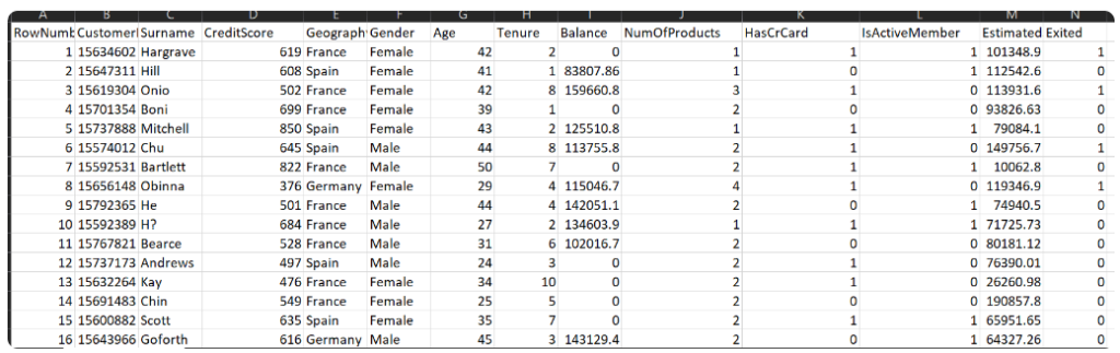
(2) List Of Independent Variables.
- RowNumber:– Represents the number of rows
- CustomerId:– Represents customerId
- Surname:– Represents the surname of the customer
- CreditScore:– Represents the credit score of the customer
- Geography:– Represents the city to which customers belong to
- Gender:– Represents Gender of the customer
- Age:- Represents age of the customer
- Tenure:- Represents tenure of the customer with a bank
- Balance:- Represents balance held by the customer
- NumOfProducts:- Represents the number of bank services used by the customer
- HasCrCard:- Represents if a customer has a credit card or not.
- IsActiveMember:- Represents if a customer is an active member or not
- EstimatedSalary:- Represents the estimated salary of the customer
- Exited:- Represents if a customer is going to exit the bank or not.
(3) Importing Necessary Libraries For ANN.
import numpy as numpy
import pandas as pandas
import tensorflow as tf
import tensorflow
from tensorflow import keras
from tensorflow.keras import Sequential
from tensorflow.keras.layers import Dense
(4) Import Data Set
data = pd.read_csv('Churn_Modelling.csv')
data.shape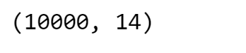
(5) Generating Required Input Features (X)
X = data.iloc[:,3:-1]
print(X)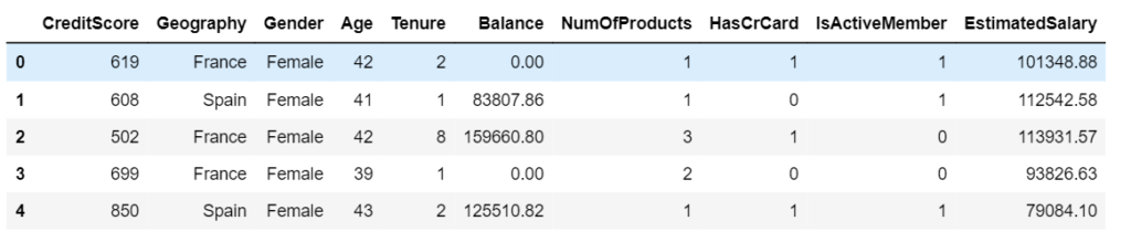
(6) Generating Dependent Variable Vector (Y)
Y = data.iloc[:,-1]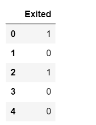
(7) Encoding Categorical Variable Gender
- Here our gender column has only 2 categories which are male and female, we are going to use LabelEncoding.
- This type of encoding will simply convert this column into a column having values of 0 and 1.
- In order to use Label Encoding, we are going to use the LabelEncoder class from sklearn library.
from sklearn.preprocessing import LabelEncoder
LE1 = labelEncoder()
X['Gender'] = np.array(LE1.fit_transform(X['Gender']))
X.head()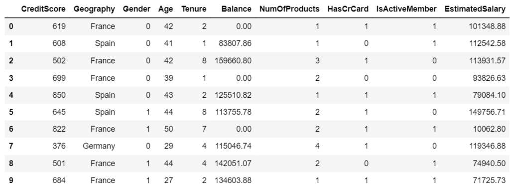
(7) Encoding Categorical Variable Geography
- The country column has France, Germany, and Spain.
- We can use Label Encoding here and directly convert those values into 0,1,2 like that. However, once those values are encoded, they will be converted into 0,1,2. Here the issue is algorithm will assume higher numbers are more important.
- In one hot encoding, all the string values are converted into binary streams of 0’s and 1’s. One-hot encoding ensures that the machine learning algorithm does not assume that higher numbers are more important.
X = pd.get_dummies(X, columns=['Geographu'], drop_first= False, dtype=int)
X.head()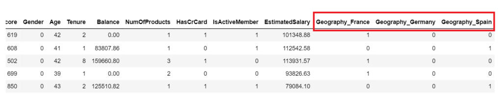
(8) Splitting Dataset Into Training & Testing Set
from sklearn.model_selection import train_test_split
X_train, X_test, Y_train, Y_test = train_test_split(X, y, test_size = 0.2, random_state = 0)
print('Training Set:',X_train.shape)
print('Testing Set:', X_test.shape)
print('Training Set:',Y_train.shape)
print('Testing Set:', Y_test.shape)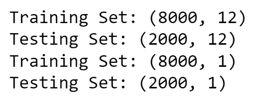
(8) Performing Feature Scaling.
- The very last step in our feature engineering phase is feature scaling. It is a procedure where all the variables are converted into the same scale.
- Sometimes in our dataset, certain variables have very high values while certain variables have very low values. So there is a chance that during model creation, the variables having extremely high value dominate variables having extremely low value.
- Because of this, there is a possibility that those variables with the low value might be neglected by our model, and hence feature scaling is necessary.
Note:
- Now here I am going to answer one of the most important questions asked in a machine learning interview.
- ” When to perform feature scaling – before the train-test split or after the train-test split?”.
- Well, the answer is after we split the dataset into training and testing datasets. The reason is, that the training dataset is something on which our model is going to train or learn itself.
- The testing dataset is something on which our model is going to be evaluated.
- If we perform feature scaling before the train-test split then it will cause information leakage on testing datasets which neglects the purpose of having a testing dataset hence we should always perform feature scaling after the train-test split.
- Whenever standardization is performed, all values in the dataset will be converted into values ranging between -3 to +3.
- While in the case of normalization, all values will be converted into a range between -1 to +1.
- There are few conditions on which technique to use and when. Usually, Normalization is used only when our dataset follows a normal distribution while standardization is a universal technique that can be used for any dataset irrespective of the distribution. Here we are going to use Standardization.
from sklearn.preprocessing import StandardScaler
sc = StandardScaler()
X_train = sc.fit_transform(X_train)
X_test = sc.fit_transform(X_test)
(9) Initializing Artificial Neural Network
- This is the very first step in creating ANN.
- Here we are going to create our ANN object by using a certain class of Keras named Sequential.
ann = tf.keras.models.Sequential()(10) Creating Input Layer
First Layer Role: The first layer in a neural network is where your model first encounters the input data. It’s like the entrance to a building; it’s where you first step inside.
Knowing the Data Size: The
input_dim=12part tells the first layer how many pieces of information (or features) each data point has. In other words, it informs the model about the size of the input data. This is crucial because the model needs to know the “shape” of the data it’s working with.Setting the Stage: Think of it as setting up the workspace for the workers (neurons) in the first layer. By specifying
input_dim=12, you’re saying, “Hey, workers, get ready to handle data with 12 features.” This way, the workers know what to expect and can process the data correctly.Propagation: As data flows through the network, each layer needs to know what to expect from the previous one. The first layer sets the stage by specifying the input size, and subsequent layers automatically know what to expect because they’re connected.
- So, in simple terms,
input_dim=12is like telling the first layer of your neural network the size of the data it will be dealing with. It’s an essential step to ensure that the model processes the data accurately as it flows through the network.
model.add(Dense(20, activation='relu', input_dim=12))(11) Creating Second Hidden Layer
- Second Layer: You’re adding a second step with 20 workers (neurons). Each worker focuses on different aspects of the problem, just like having different experts for different parts of the task. The ‘relu’ activation means that each worker decides whether their contribution to the solution should be positive or zero.
model.add(Dense(20,activation='relu'))(12) Creating Third Hidden Layer
- Third Layer: Now, you’re adding a third step, also with 20 workers. These workers continue to break down the problem into finer details. It’s like having even more experts who specialize in different aspects of the task.
model.add(Dense(20,activation='relu'))Hidden Layers:
- These additional layers you’re adding are called “hidden layers.” They’re called “hidden” because they’re between the input and the final output, and they help the model learn complex patterns in the data.
How Many Hidden Layers Can we Add?
The number of hidden layers you can add depends on the complexity of the problem we are trying to solve and the amount of data we have. In simple problems, a few hidden layers may be enough. However, for more complex tasks or large datasets, you might need more hidden layers to capture intricate patterns.
There’s no one-size-fits-all answer. It’s often a matter of experimentation and finding the right balance. Too many layers can lead to overfitting (memorizing data instead of learning patterns), and too few layers may not capture enough complexity. It’s like deciding how many experts we need for a challenging task—sometimes we need more, and sometimes we need fewer, depending on the task’s difficulty.
(13) Creating Output Layer
Final Layer: This is the last step in our problem-solving process, like the final decision or answer to a question.
Single Unit (Neuron): The 1 unit means that this step has only one worker (neuron). It’s like the ultimate decision-maker in our process.
Sigmoid Activation: The sigmoid activation function used here is like a worker who makes a binary decision. It’s often used for problems where we have two choices or classes, like “yes” or “no,” “spam” or “not spam.” This worker decides which of the two choices is the most likely answer.
model.add(Dense(1, activation='sigmoid'))(14) Displaying Model Summary
model.summary()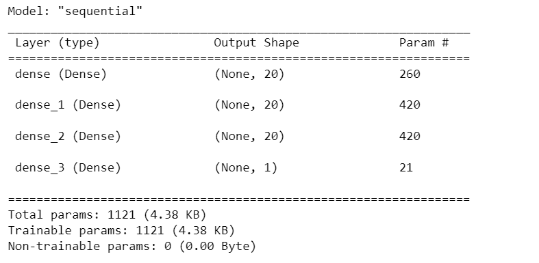
(15) Compiling Artificial Neural Network
- We have now created layers for our neural network.
- In this step, we are going to compile our ANN.
Optimizer (Adam): Think of the optimizer as the “smart worker” responsible for improving the model’s performance. It’s like a factory manager who makes adjustments to the workers (neurons) to make them better at their jobs. “Adam” is a specific optimization algorithm that’s good at fine-tuning the model.
Loss (binary_crossentropy): The loss function measures how well the model is doing its job. It’s like a quality control inspector who checks the products coming out of the factory and gives a score based on how accurate they are. “binary_crossentropy” is a type of score used when the task is to classify things into two categories, like “yes” or “no.”
Metrics (accuracy): Metrics are like the performance indicators of the factory. “Accuracy” is one such indicator, and it measures how many products (predictions) the factory got right out of all the products it made. It’s like calculating the percentage of correct answers on a test.
- So, when we compile the model with these settings, we are essentially telling it how to improve itself (optimizer), how to measure its performance (loss function), and what performance indicators to pay attention to (metrics).
- It’s like giving instructions to a factory manager on how to make the workers better at their jobs and how to assess the quality of the products they produce.
model.compile(optimizer='Adam', loss='binary_crossentropy', metrics=['accuracy'])(16) Training Neural Network Model
Input Data (X_train): These are the features or input variables used to train the neural network. Each row represents an example, and each column represents a feature.
Target Outputs (y_train): These are the corresponding target values or labels that the network is trying to predict based on the input data. Each value in y_train corresponds to an example in X_train.
Batch Size (50): During training, instead of processing all training examples at once, we split them into smaller groups or batches, each containing 50 examples. This is done to make the optimization process more efficient and to fit the data into memory.
Epochs (100): The training process is divided into 100 epochs. In each epoch, the entire training dataset (all examples) is processed by the neural network. This repetition helps the network learn from the data through iterative adjustments of its parameters.
Verbose (1): The verbose parameter controls the amount of information displayed during training. A setting of 1 means that training updates will be printed to the console, providing information about the progress of each epoch.
Validation Split (0.2): A portion of the training data (20%) is set aside for validation purposes. During training, the network’s performance on this validation set is monitored to assess how well it generalizes to unseen data.
- Model Fitting: The model.fit function executes the training process, which involves repeatedly passing batches of input data through the neural network, computing predictions, comparing them to the target outputs, adjusting the network’s internal parameters (weights and biases), and repeating this process for the specified number of epochs.
- The goal of this entire process is to optimize the neural network’s parameters so that it can make accurate predictions on new, unseen data (generalization) based on the patterns it learns from the training data.
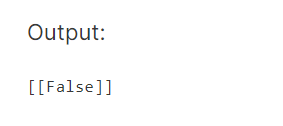
history = model.fit(X_train, y_train, batch_size = 50, epochs=100, verbose=1, validation_split=0.2)(17) Predicting Result for Single Point Observation
print(ann.predict(sc.transform([[1, 0, 0, 600, 1, 40, 3, 60000, 2, 1, 1,50000]])) > 0.5)